Download
1 / 31
310 likes | 381 Views
Top k Knapsack Joins and Closure Early Results. Witold LITWIN & Thomas Schwarz U. Paris Dauphine, France witold.litwin@dauphine.fr Santa Clara U., CA, tjschwarz@scu.edu. Knapsack Join (KS-Join). The join defined by the sum of the join attributes being at most some constant

E N D
Top k Knapsack Joins and Closure Early Results Witold LITWIN & Thomas Schwarz U. Paris Dauphine, France witold.litwin@dauphine.fr Santa Clara U., CA, tjschwarz@scu.edu
Knapsack Join (KS-Join) • The join defined by the sum of the join attributes being at most some constant • Father of 4 kids wishing to buy toys for at most 100€ total • A person wishing to buy a computer tower, a screen, a printer and a desk for at most 1000 € • ….
Knapsack Join (KS-Join) • Traditional join • R1 Join R2 on c1 = c2 • KS - join • R1 Join R2 on c1 + c2 ≤ C • Syntax legal for FROM clause in Access, SQL Server…
Top k Knapsack Join (KS-Join) • Top k items with respect to the descending order on the constant • Usually, only a few items the most close to the constant are of interest • Select TOP 1 * from Toys T1, Toys T2, Toys T3, Toys T4 Where T1.Price + T2.Price + T3.Price + T4.Price ≤ 100 and T1.Id < T2.Id and T2.Id < T3.Id and T3.Id < T4.Id Order by T1.Price + T2.Price + T3.Price + T4.Price Desc;
Top k Knapsack Join (KS-Join) • Top k Knapsack joins are of obvious interest • How DBMSs deal with ? • Nested loop • To our best knowledge • Result: execution time makes the SQL capability useless for a larger data set • Consider our example for just 1000 toys to choose from • FYI, 1K-tuple table & 3-way KS-join killed SQL Server
Our Goal : Optimizing Top k KS-Joins • Algorithms provably faster than usual nested loop • Formulate the algorithm • Prove the complexity, storage & processing costs • KS-optimized Nested Loop • Self-join Nested Loop • Sort Merge • KS – Join Indices • Distributed KS – Join Indices
Our Goal : Optimizing Top k KS-Joins • Early Results • Only for Top k KS-Joins (TkKS-Joins) • Only the formal analysis as yet • Many variants of TkKS-Join queries left for future work • See the paper
KnapsackProblem (KP) • NP-hard optimization problem • Among most studied • Input: • A set O of objects {o1,...on} • An m-d subspace called knapsackK with • values bi, 1 ≤ i ≤ m, represent each the i-th dimension's capacity of the knapsack • Vector cjrepresents the benefit of the object jif in the knapsack
KnapsackProblem (KP) • Input (continued): • The knapsack's constraints matrix with entries ai,j ; 1 ≤ j ≤ n ; • Each entry stores the constraint value for each object j in each dimension i(price, size, volume...). • Output: • Aset O'of objects stored in the knapsack.
KnapsackProblem (KP) • Binary variablexj; xj{0, 1}, indicates the selection of the object j into the knapsack • (x j= 1) for object j in and (xj = 0) otherwise • xjis 0–1 decision variable
KnapsackProblem (KP) • Select the elements of O’ which maximize the total profit of the selected objects • Provided the match of the knapsack constraints
KnapsackProblem (KP) • Formally, maximize: • Subject to:
KnapsackProblem (KP) • The most frequently investigated case is the 1-d one • I.e.,i= 1 • Often, or perhaps even the most often, the KP concept designates implicitly this case. • Frequently, in addition, one also sets every cj to cj = aj. • Both conditions are ours below • unless we state otherwise • The m-d one is referred to then, if needed, as multidimensional (MKP).
KnapsackProblem (KP) • The general research orientation for KP and MKP • Find a heuristic providing acceptable approximate result • For the possibly largest data set • In the fastest time, • Or acceptable time • Given necessary constraints on the computer system used.
KP / TkKS -Join • Our research orientation follows the database approach • Find an exact result • For a reasonably practical problem subspace • For a database size data • Say, 1Ktuples per table at least
KP / TkKS -Join • Find an exactresult (continued) • In the fastest time • Or acceptable time • Minutes at most • Given necessary constraints on the computer system used • Mainly storage cost
KnapsackProblem (KP) • Our reasonably practical problem subspace at present: • As we already stated cj = aj • 1-d space • Fixed # of objects for the knapsack • Join instead of closure
KnapsackProblem (KP) • Our reasonably practical problem subspace at present (continued): • One tuple = one potential selection • One object = one tuple with distinct ID • No objects selected twice in a tuple for the knapsack • Closure, MKP… left for the future
Nested loop TkKS-Join • Basic cost for tables withn1…nm tuples • O (n1*…*nm) • To accelerate the calculus start with: • Evaluation of the restrictions ti < C • Evaluation of ti ≤ C – (Min1+…+Minj+…+Minm) • for any j ≠ i • DBMS may easily maintain the Minjstatistics • Cost can be O(m) or even O (1) only • Idem for C ≥ Max1+…+Maxm ?
Nested loop TkKS-Join • Self-joint of a table with its copies • Since KS-join is commutative one may avoid doubles • E.g. if we have tuple (t1, t2) then we should not have the tupletuples (t2, t1) • In general, we need only one tuple from all its permutations • The optimizing cuts the complexity and calculus time by half, at least • Final word: we may have • O (n1*…*nm /S), where S ≥ 1
150 C =150 150 Sort-Merge TkKS-Join • 2-wayjoin
Sort-Merge TkKS-Join • Processing cost of 3-way TkKS-Join • O (n1+n2) in general • O ((n1+n2)/2) for self-join • For n-way TkKS-Join • O (nm*…n3(n2 + n1)) in general • For self-join ? • E.g. For 16K-tuple R1 and R2tables m-way join accelerates 8K times • 1sec instead of 2+ hours • See the paper
KS-Join Index • A relational table IKS with at least the attributes (C, t1.Id,…,tm.Id) • Here C = t1.c+…+tm.c • Also t1.Id <… <tm.Id • Can be also seen as a materialized view • Some or all ti.c should be useful as well • E.g. for queries with additional restrictions on individual prices
KS-Join Index • IKS should be implemented as file sorted on C first • Then, on other key or non-key attributes of interest • E.g., a B-tree or trie… • Storage cost: • O (n1*…*nm) in general • Half of it or less for copies of the same table • 3-way indices may be in RAM • More should be typically on flash or disk
KS-Join Index • Processing cost • O (Log p (n1*…*nm) ) or less, according to the storage cost, where p is the tree fan-out • Expected practical figures • ms for RAM, e.g., 3-way KS-Join index for 1K-tuple tables • under 10 ms for flash • under 100 ms for the disk, e.g., 4-way KS-Join index for our 1K-tuple tables
KS-Join Index • Maintainance cost • High processing cost • E.g., 1 insert into our 1K tables generates 1M new entries • Main drawback of KS-Indices at present • Efficient processing is an open problem
Composing KS-Join Indices • TkKS-Join calculus can compound existing KS-Indices • m-way & n-way indices may speed up (m+n)-way TkKS Join • Through the sort-merge algorithm applied to both indices • Seconds may suffice for up to 6-way joins • E.g., for our 1K relations
Scalable-Distributed TkKS-Join Index • Speeds up the calculus of even larger joins • Using the parallel distributed processing • Dozens of seconds may suffice for an 8-way join • Over our favorite 1Ktuple relations • With two 4-way KS-Indices • Each being distributed over 1K nodes • Through, e.g., RP* SDDS • Maintainance time speeds-up as well
100 350 800 9900 10 50 450 700 Scalable-Distributed TkKS-Join Index • C = 900 ; arrows show nodes to join in parallel
Conclusion • TkKS-Joins are potentially useful • Our optimizations may speed up the processing by orders of magnitude • Queries with TkKS-Joins become then practical • With all the usual disclaimers, the results appear ready for mainstream DBMSs
Future Work • Deeper formal analysis • Experiments • More TkKS-Join query types • See the paper Thank You for Your Attention