Download
1 / 20
200 likes | 292 Views
Learn how to calculate t-scores for hypothesis testing in statistics, including defining hypotheses and conducting t-tests. Understand the critical ratio, error variance, and obtaining t-values.

E N D
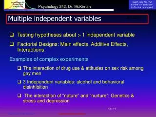
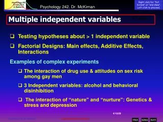
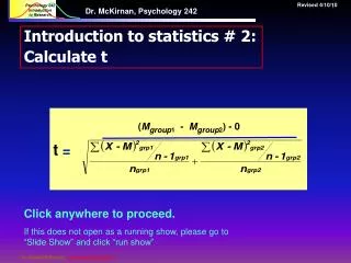
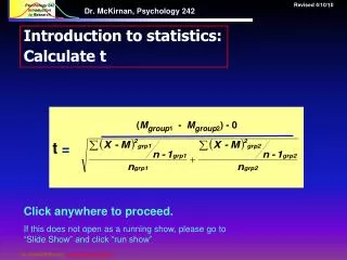
Revised 4/10/10 (Mgroup1 - Mgroup2) - 0 t = Dr. McKirnan, Psychology 242 Introduction to statistics: Calculate t Click anywhere to proceed. If this does not open as a running show, please go to “Slide Show” and click “run show”
Statistical Hypothesis Testing • We use the t test (or any statistic) to test our hypothesis. • Part of the operational definition of our variables is the numbers we use to represent them. • What is our (statistical) hypothesis? • That the mean score (M) for the experimental group is greater than (or less than…) the M for the control group… • …by more than we might expect by chance alone. • What is the “null” hypothesis? • Any difference between the M for the experimental group and the M for the control group is by chance alone. • Mexperimental– Mcontrol = 0, except for chance (error variance) The research question (in statistical terms): • In our study, is the difference between the group Means (Mexp – Mcontrol)greater than (or less than…)0 by more than we would expect by chance alone?
Statistical Hypothesis Testing The concept underlying the t test is the critical ratio: How strongly did the independent variable affect the outcome? How much error variance [“uncertainty”, “noise”] is there in the data For a t-test: The experimental effect is the difference between the Ms of the experimental & control groups The error variance is the square root of the summed variances of the groups, similar to a two-group standard deviation. (Mexp- Mcontrol) - 0 =t =
(Mgroup1 - Mgroup2) - 0 t = (Mgroup1 - Mgroup2) - 0 t = t-test (Mgroup1 - Mgroup2) - 0 t = Difference between groups standard error of M = • How strong is the experimental effect? • How much error variance is there
(Mgroup1 - Mgroup2) - 0 t = t-test (Mgroup1 - Mgroup2) - 0 t = Difference between groups standard error of M = • Standard error: • Calculate the variance for for group 1 • Sum of squares • Divided by degrees of freedom (n-1) • Divide by n for group 1 • Repeat for group 2 • Add them together • Take the square root
(Mgroup1 - Mgroup2) - 0 t = (Mgroup1 - Mgroup2) - 0 t = t-test (Mgroup1 - Mgroup2) - 0 t = Difference between groups standard error of M = The expanded version…
(Mgroup1 - Mgroup2) - 0 t = Compute a t score • Compute the Experimental Effect: • Calculate the Mean for each group, subtract Mgroup2from Mgroup1. • Compute the Standard Error • Calculate the variance for each group
Calculate the Variance using the box method: 1. Enter the Scores. X 7 6 2 1 4 1 7 4 2 6 M4 4 4 4 4 4 4 4 4 4 X - M 3 2 -2 -3 0 -3 3 0 -2 2 Σ = 0 (X - M)2 9 4 4 9 0 9 9 0 4 4 Σ = 52 2. Calculate the Mean. 3. CalculateDeviation scores: Simple deviations: Σ(X – M) = 0 Square the deviations to create + values: ΣSquares = Σ(X - M)2 = 52 4. Degrees of freedom: df = [n – 1] = [10 – 1] = 9 5. Apply the Varianceformula: n= 10 Σ= 40 M = 40/10 = 4
(Mgroup1 - Mgroup2) - 0 t = Compute a t score effect error • Compute the Experimental Effect: • Calculate the Mean for each group, subtract group2M from group1M. • Compute the Standard Error • Calculate the variance for each group • Divide each variance by n for the group • Add those computations • Take the square root of that total • Compute t • Divide the Experimental Effect by the Standard Error
Examples of deriving t values M = 2.5 M = 4 M1 – M2 = 4 – 2.5 = 1.5 Standard error = .75 t = = = 2 M1 – M2 = 4 – 2.5 = 1.5 Standarderror = 1.75 t = = = .86 1.5 1.75 1.5 .75 M = 2.5 M = 4
Clicker! Why does this have a t value = 2? • The variance within each group is large relative to the difference between the group means. • The M of the larger group = 4 and there are 2 groups • The difference between the group means is large relative to the variance within each group • t is a random number M = 2.5 M = 4
Clicker! Why does this have a t value = 2? • The variance within each group is large relative to the difference between the group means. • The M of the larger group = 4 and there are 2 groups • The difference between the group means is large relative to the variance within each group • t is a random number M = 2.5 M = 4
Clicker, 2 Why does this have a t value = .86? • The variance within each group is large relative to the difference between the group means. • The M of the larger group = 4 and there are 2 groups • The difference between the group means is large relative to the variance within each group • t is a random number M = 2.5 M = 4
Clicker, 2 Why does this have a t value = .86? • The variance within each group is large relative to the difference between the group means. • The M of the larger group = 4 and there are 2 groups • The difference between the group means is large relative to the variance within each group • t is a random number M = 2.5 M = 4
Sampling distribution & statistical significance • Any 2 group Ms differ at least slightly by chance. • Any t score is therefore > 0 or < 0 by chance alone. • We assume that a t score with less than 5% probability of occurring [p < .05] is not by chance alone • We calculate the probability of a t score by comparing it to a sampling distribution Sampling distribution of t scores
The Sampling Distribution -3 -2 -1 0 +1 +2 +3 Z or t Scores (standard deviation units) We can segment the population into standard deviation unitsfrom the mean. These are denoted as Z or t M = 0, 34.13% of scores from Z = 0 to Z = +1 and from Z = 0 to Z = -1 each standard deviation represents Z = 1 13.59% of scores + 13.59% of scores Each segment takes up a fixed % of cases (or “area under the curve”). 2.25% of scores + 2.25% of scores
t scores and statistical significance, 1 t = = = 2 t = 2.0 Comparing t to a sampling distribution: About 98% of t values are lower than 2.0 M1 – M2 = 4 – 2.5 Standard error About 98% of t scores 1.5 .75 Sampling distribution of t scores
t scores and statistical significance, 1 1.5 1.75 M1 – M2 = 4 – 2.5 Standarderror = = t = .86 t = .88 About 81% of the distribution of t scores are below .88. (area under the curve = .81) About 81% of scores Sampling distribution of t scores
Between v. within group variance: t-test logic The difference between Ms is the same in the two data sets. t = .86 t = 2.0 Since the variances differ… • We get different t values • We make differ judgments about whether these t scores occurred by chance. About 98% of t scores; p < .05 About 81% of scores Sampling distribution of t scores
Continue… Continue this series by clicking on the module for The Central Limit Theorem.