Understanding Seismic Events

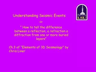
1. Understanding Seismic Events Or “ How to tell the difference between a reflection, a refraction a diffraction from one or more buried layers” Ch.3 of “Elements of 3D Seismology” by Chris Liner

2. Outline-1 • Full space, half space and quarter space • Traveltime curves of direct ground- and air- waves and rays • Error analysis of direct waves and rays • Constant-velocity-layered half-space • Constant-velocity versus Gradient layers • Reflections • Scattering Coefficients

3. Outline-2 • AVA-- Angular reflection coefficients • Vertical Resolution • Fresnel- horizontal resolution • Headwaves • Diffraction • Ghosts • Land • Marine • Velocity layering • “approximately hyperbolic equations” • multiples

4. A few NEW and OLD idealizations used by applied seismologists…..

5. IDEALIZATION #1: “Acoustic waves can travel in either a constant velocity full space, a half-space, a quarter space or a layered half-space”

6. A full space is infinite in all directions -z -X X z

7. A half-space is semi-infinite X -X z

8. A quarter-space is quarter-infinite X -X z

9. Outline • Full space, half space and quarter space • Traveltime curves of direct ground- and air- waves and rays • Error analysis of direct waves and rays • Constant-velocity-layered half-space • Constant-velocity versus Gradient layers • Reflections • Scattering Coefficients

10. A direct air wave and a direct ground P-wave ….. X -X z

11. A direct air wave and a direct ground P-wave …..

12. A direct air wave and a direct ground P-wave …..

13. A direct air wave and a direct ground P-wave …..

14. The data set of a shot and its geophones is called a shot gather or ensemble. Vp air ray wavefront Vp ground geophone

15. Traveltime curves for direct arrivals Shot-receiver distance X (m) Time (s)

16. Traveltime curves for direct arrivals Shot-receiver distance X (m) Direct ground P-wave e.g. 1000 m/s Time (s) dT dx Air-wave or air-blast (330 m/s) dT dx

17. Outline • Full space, half space and quarter space • Traveltime curves of direct ground- and air- waves and rays • Error analysis of direct waves and rays • Constant-velocity-layered half-space • Constant-velocity versus Gradient layers • Reflections • Scattering Coefficients

18. Error analysis of direct waves and rays See also http://www.rit.edu/cos/uphysics/uncertainties/Uncertaintiespart2.html by Vern Lindberg

19. TWO APPROXIMATIONS TO ERROR ANALYSIS • Liner presents the general error analysis method with partial differentials. • Lindberg derives the uncertainty of the product of two uncertain measurements with derivatives.

20. Error of the products • “The error of a product is approximately the sum of the individual errors in the multiplicands, or multiplied values.” V = x/t x = V. t where, are, respectively errors (“+ OR -”) in the estimation of distance, time and velocity respectively.

21. Error of the products • “The error of a product is approximately the sum of the individual errors in the multiplicands, or multiplied values.” (1) Rearrange terms in (1) (2) Multiply both sides of (2) by V (3) Expand V in (3) (4) Note that (5) is analogous to Liner’s equation 3.7, on page 55 (5)

22. Error of the products “In calculating the error, please remember that t, x and V and x are the average times and distances used to calculate the slopes, i.e. dT and dx below (1 + error in x } } + error in t } - error in t } Time (s) - error in x dT dx dT dx Region of total error

23. Traveltime curves for direct arrivals Shot-receiver distance X (m) Direct ground P-wave e.g. 1000 m/s Time (s) dT dx Air-wave or air-blast (330 m/s) dT dx

24. Outline • Full space, half space and quarter space • Traveltime curves of direct ground- and air- waves and rays • Error analysis of direct waves and rays • Constant-velocity-layered half-space • Constant-velocity versus Gradient layers • Reflections • Scattering Coefficients

25. A layered half-space X -X z

26. A layered half-space with constant-velocity layers Eventually, …..

27. A layered half-space with constant-velocity layers Eventually, …..

28. A layered half-space with constant-velocity layers Eventually, …..

29. A layered half-space with constant-velocity layers ………...after successive refractions,

30. A layered half-space with constant-velocity layers …………………………………………. the rays are turned back top the surface

31. Outline • Full space, half space and quarter space • Traveltime curves of direct ground- and air- waves and rays • Error analysis of direct waves and rays • Constant-velocity-layered half-space • Constant-velocity versus gradient layers • Reflections • Scattering Coefficients

32. Constant-velocity layers vs. gradient-velocity layers “Each layer bends the ray along part of a circular path”

33. Outline • Full space, half space and quarter space • Traveltime curves of direct ground- and air- waves and rays • Error analysis of direct waves and rays • Constant-velocity-layered half-space • Constant-velocity versus gradient layers • Reflections • Scattering Coefficients

35. Direct water arrival

36. Hyperbola y asymptote x x As x -> infinity, Y-> X. a/b, where a/b is the slope of the asymptote

37. Reflection between a single layer and a half-space below O X/2 X/2 V1 h P Travel distance = ? Travel time = ?

38. Reflection between a single layer and a half-space below O X/2 X/2 V1 h P Travel distance = ? Travel time = ? Consider the reflecting ray……. as follows ….

39. Reflection between a single layer and a half-space below O X/2 X/2 V1 h P Travel distance = Travel time =

40. Reflection between a single layer and a half-space below Traveltime = (6)

41. Reflection between a single layer and a half-space below and D-wave traveltime curves asymptote Matlab code

42. Two important places on the traveltime hyperbola #1 At X=0, T=2h/V1 T0=2h/V1 * h Matlab code

43. #1As X--> very large values, and X>>h , then (6) simplifies into the equation of straight line with slope dT/dx = V1 If we start with (6) as the thickness becomes insignificant with respect to the source-receiver distance

44. By analogy with the parametric equation for a hyperbola, the slope of this line is 1/V1 i.e. a/b = 1/V1

45. What can we tell from the relative shape of the hyperbola? 3000 Increasing velocity (m/s) 1000 50 Increasing thickness (m) 250

46. “Greater velocities, and greater thicknesses flatten the shape of the hyperbola, all else remaining constant”

47. Reflections from a dipping interface #In 2-D Direct waves 30 10 Matlab code

48. Reflections from a 2D dipping interface #In 2-D: “The apex of the hyperbola moves in the geological, updip direction to lesser times as the dip increases”

49. Reflections from a 3D dipping interface #In 3-D Azimuth (phi) strike Dip(theta)

50. Reflections from a 3D dipping interface #In 3-D Direct waves 90 0 Matlab code