Download
1 / 74
740 likes | 968 Views
Burst Exponents in Stochastic Modeling Experiments of Hydraulic Fracture. Bjørn Skjetne 1 and Alex Hansen 1 1 Department of Physics Norwegian University of Science and Technology (NTNU) N-7491 Trondheim Norway. Motivation.

E N D
Burst Exponents in Stochastic Modeling Experiments of Hydraulic Fracture Bjørn Skjetne1and Alex Hansen1 1Department of Physics Norwegian University of Science and Technology (NTNU) N-7491 Trondheim Norway
Motivation • CCS – currently great interest in how one should go about in order to facilitate Carbon Capture and Storage. Politicians and environmentalists place a lot of emphasis on this. It is the storage of carbon that concerns us in the context of hydraulic fracture. • Hydraulic fracture is a well known method to enhance oil and gas production. Interest in this approach is increasing as the remaining oil becomes more difficult to extract. Also has an environmental side, since a lot of attention has been focused on pollution from oil extraction operations. • Physics. Hydraulic fracture also represents an interesting phenomenon from the academic point of view. Here we can test to what extent our physical understanding of fracture and flow tallies with experimental reality.
Our project • CCS, concerns geologic storage of CO2. A grant from the Norwegian Research Council via their CLIMIT program for the project ‘Efficient CO2 Absorption in Water-Saturated Porous Media through Hydraulic Fracture’. This is a joint project between SINTEF and NTNU.
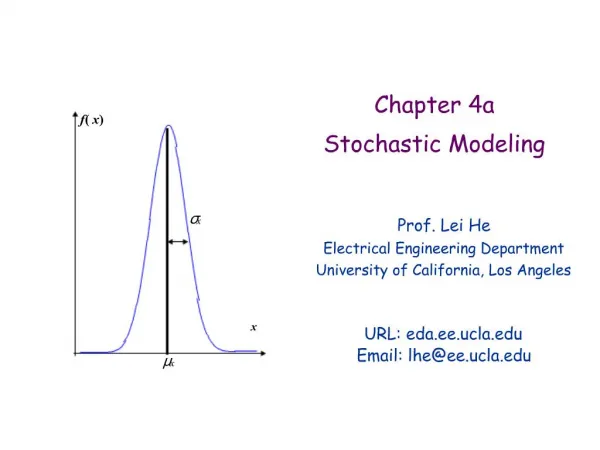
Stochasticmodelingoffracture KEY FEATURES: • Assumption of a meso-scale, intermediate between the macroscopic and the microscopic scales. • Discretize the system on a regular lattice. • Define the forces between the nodes on the lattice. • Introduce a driving force in the system in the form of a potential gradient or a boundary condition. • Define a breaking rule which specifies when and where damage should occur. • Specify a consistent stopping criterion.
Biot’stheoryof linear poroelasticity In our problem we need to understand the behaviour of fluid-saturated porous media. Hence we introduce the concept of a POROELASTIC ELEMENT. It is a solid matrix which is permeated by a network of connected pores. What is the mechanical behaviour of such an entity? A well known relationship between stress and strain is In analogy with this Maurice Biot (1941) introduced a similar quantity for the fluid response, i.e.,
Biot’stheoryof linear poroelasticity In our problem we need to understand the behaviour of fluid-saturated porous media. Hence we introduce the concept of a POROELASTIC ELEMENT. It is a solid matrix which is permeated by a network of connected pores. What is the mechanical behaviour of such an entity? Maurice Biot coupled the two equations to obtain two constitutive equations: Essentially, this is Biot theory in a nutshell! From this assumption we can deduce governing equations of FLUID FLOW and MECHANICAL EQUILIBRIUM.
Fluid flow in Biottheory In hydraulic fracture fluid is injected at high pressure in a well-bore and due to this fluid flows through the system. What balances the flow as the resulting potential gradient is a frictional force between the fluid and the pore walls. The average fluid velocity is then Since this is the relative movement of the fluid with respect to the solid, this can also be stated as
Fluid flow in Biottheory We regard a small poroelastic element, or control volume, through which fluid flows The volume of the fluid which enters on the left-hand side is and that which exits on the right-hand side is Consequently, the change in the fluid content is given by
Fluid flow in Biottheory We regard a small poroelastic element, or control volume, through which fluid flows We then get where we have assumed that the porosity is the same throughout the control volume. Next, we have for the right-hand side
Fluid flow in Biottheory We regard a small poroelastic element, or control volume, through which fluid flows This results in Considering all three spatial directions and adding the contributions, we get where our control volume is
Fluid flow in Biottheory We regard a small poroelastic element, or control volume, through which fluid flows Next we use the definition of Biot’s increment in fluid content which now gives Considering the time derivative of this we get
Fluid flow in Biottheory We regard a small poroelastic element, or control volume, through which fluid flows Now we make use of the expression above and obtain We now use Darcy’s Law to obtain
Fluid flow in Biottheory If we now substitute for the increment in fluid content, given by one of Biot’s constitutive equations, then we have This is the GOVERNING EQUATION OF FLUID FLOW in our system. Mechanicalequilibrium in Biottheory For the mechanical equilibrium the coupling of the expressions at the beginning also result in the addition of an extra term. The standard expression in classical elasticity becomes This is the GOVERNING EQUATION OF MECHANICAL EQUILIBRIUM.
Discretization of themodel In order to create a model of hydraulic fracture which the computer can understand we assume the material properties to be embedded in a discrete manner and in a way which allows any of these discrete points to have a consistent address. An obvious choice would be a square lattice due to its simple geometry. However, such a lattice does not have the proper macroscopic behaviour and we must choose a lattice with TRIANGULAR TOPOLOGY.
Discretization of themodel In order to create a model of hydraulic fracture which the computer can understand we assume the material properties to be embedded in a discrete manner and in a way which allows any of these discrete points to have a consistent address. An obvious choice would be a square lattice due to its simple geometry. However, such a lattice does not have the proper macroscopic behaviour and we must choose a lattice with TRIANGULAR TOPOLOGY.
Discretization of themodel In order to create a model of hydraulic fracture which the computer can understand we assume the material properties to be embedded in a discrete manner and in a way which allows any of these discrete points to have a consistent address. An obvious choice would be a square lattice due to its simple geometry. However, such a lattice does not have the proper macroscopic behaviour and we must choose a lattice with TRIANGULAR TOPOLOGY.
Discretization of themodel In order to create a model of hydraulic fracture which the computer can understand we assume the material properties to be embedded in a discrete manner and in a way which allows any of these discrete points to have a consistent address. An obvious choice would be a square lattice due to its simple geometry. However, such a lattice does not have the proper macroscopic behaviour and we must choose a lattice with TRIANGULAR TOPOLOGY.
Discretization of themodel In order to create a model of hydraulic fracture which the computer can understand we assume the material properties to be embedded in a discrete manner and in a way which allows any of these discrete points to have a consistent address. An obvious choice would be a square lattice due to its simple geometry. However, such a lattice does not have the proper macroscopic behaviour and we must choose a lattice with TRIANGULAR TOPOLOGY.
Discretization of themodel In order to create a model of hydraulic fracture which the computer can understand we assume the material properties to be embedded in a discrete manner and in a way which allows any of these discrete points to have a consistent address. In modeling hydraulic fracture we assume that our crack will propagate outward from the center of the system towards the boundaries. We introduce therefore introduce a ‘well-bore’ at the center of the lattice by removing a link.
Discretization of themodel In order to create a model of hydraulic fracture which the computer can understand we assume the material properties to be embedded in a discrete manner and in a way which allows any of these discrete points to have a consistent address. Due to the radial symmetry of the problem, we would ideally like to have a more or less circular geometry. As an approximation to this we choose a HEXAGONAL shape for the outer boundary.
Discretization of themodel In order to create a model of hydraulic fracture which the computer can understand we assume the material properties to be embedded in a discrete manner and in a way which allows any of these discrete points to have a consistent address. Finally, the underlying structure where our hydraulic fracture modeling takes place looks like this.
Specifyingforcesbetween nodes The discretization in our model is in terms of a DEFORMABLE lattice. Hence the forces between the nodes must be defined in terms of displacements. On a triangular lattice there are six neighbours to each node. These are numbered from one to six, beginning with the horizontal beam which extends towards the left-hand side.
Specifyingforcesbetween nodes The discretization in our model is in terms of a DEFORMABLE lattice. Hence the forces between the nodes must be defined in terms of displacements. Forces between the nodes are defined IN ANALOGY with ELASTIC BEAMS. The beams are fastened onto each other in such a way that the angle between them (60 degrees) is preserved, even when there is a rotation at the node.
Specifyingforcesbetween nodes The discretization in our model is in terms of a DEFORMABLE lattice. Hence the forces between the nodes must be defined in terms of displacements. We place a COORDINATE SYSTEM on each node in order to keep track of the displacements.
Specifyingforcesbetween nodes The discretization in our model is in terms of a DEFORMABLE lattice. Hence the forces between the nodes must be defined in terms of displacements. The beams are assumed to be brittle-elastic and the elastic response is a combination of AXIAL, SHEAR and FLEXURAL forces. Thick beams have been assumed in the expressions derived.
Specifyingforcesbetween nodes The discretization in our model is in terms of a DEFORMABLE lattice. Hence the forces between the nodes must be defined in terms of displacements. Depending on the combination of displacements at any given point in time, the forces are calculated accordingly..
Poroelastic beams To include Biot’s theory in our model of hydraulic fracture we include in our beams the assumption that they are porous. Flow through the beams are along the axis between the nodes that it connects.
Poroelastic beams To include Biot’s theory in our model of hydraulic fracture we include in our beams the assumption that they are porous. Flow through the beams are along the axis between the nodes that it connects. To say a few words about the Biot-Willis parameter which couples in the pore pressure, this expresses how much of the bulk strain is taken up by the change in the pore volume and how much is taken up by the change in the solid volume.
Biot-Willis parameter The governing equation of mechanical equilibrium was obtained from the two constitutive equation resulting from Biot’s coupling of volumetric strain-stress with increment in fluid content-pore pressure. For the relationship between the independent variables we have The expression for the parameter which obtains in the derivation of mechanical equilibrium in the equation at the top is
Biot-Willis parameter PHYSICAL INTERPRETATION The Biot-Willis parameter is an expression of the increment in fluid content with respect to changes in volumetric strain. A number between zero and one having the following interpretation: INCOMPRESSIBLE LIQUID INCOMPRESSIBLE SOLID All the bulk strain is taken up by the change in solid volume All the bulk strain is taken up by the change in pore volume 0.79 (Berea sandstone)
Beam failurecriterion In order for our system to fracture we need to define a fracture criterion. The one we use is Here F is the axial force and M is the bending moment. Random thresholds are generated for each beam on the lattice, one for the amount of axial force that the beam can withstand, and one for the amount of bending it can withstand. These are then combined as shown. When a beam breaks it is removed irreversibly from the lattice, only retaining its axial force where relative displacements indicate local compression. Axial contribution to beam breaking is assumed to occur only when beams are loaded in tension. Disorder Thresholds are generated by raising a random number to a power D, a positive power indicates that some thresholds deviate towards weak strength. Likewise, A negative D indicates that some of the thresholds deviate towards stronger strength. The magnitude of D controls how many of the thresholds deviate in this way, i.e., how strong the disorder is.
Crack growth and disorder – uniaxial loading of a sheet with a central crack Fracture criterion: Crack tip: high stress intensity STRETCHED • No disorder: fracture is stress dominated, and crack growth localized to a single existing crack. Unstable. • Disorder: if the local variation in material strength is strong enough, new cracks will appear randomly. Fracture is disorder dominated. Stable. COMPRESSED ? L=90 lattice, longitudinal axial stresses shown
Brittle fracture in the presence of disorder Disorder is imposed on the beams in the form of random breaking thresholds. Elastic properties are assumed to be identical from one beam to the next. • Initially, cracks appear on random locations. • Some of the smaller cracks grow before being arrested by the surroundings. • A cross-over occurs from a disorder-dominated process to a stress-dominated process, where smaller cracks merge into a macroscopic crack. • Localized fracture, catastrophic crack growth, sets in.
Numericalcalculation Fracture in our model is driven by a potential gradient which is set up by injecting fluid at the center of the system. Here the pressure is kept constant throughout the fracturing process.
Numericalcalculation Fracture in our model is driven by a potential gradient which is set up by injecting fluid at the center of the system. Here the pressure is kept constant throughout the fracturing process. CONJUGATE GRADIENTS Since the expressions which we derive for the poroelastic forces in the system are all linear, the resulting elastic energy expressionis quadratic.
Numericalcalculation Fracture in our model is driven by a potential gradient which is set up by injecting fluid at the center of the system. Here the pressure is kept constant throughout the fracturing process. CONJUGATE GRADIENTS Since the expressions which we derive for the poroelastic forces in the system are all linear, the resulting elastic energy expressionis quadratic. An efficient way to minimize a quadratic form is to use conjugate gradients. The minimum in our system corresponds to that situation where on each node the sum of forces and moments is zero. Physically, this is the required situation for a system in mechanical equilibrium.
Numericalcalculation Fracture in our model is driven by a potential gradient which is set up by injecting fluid at the center of the system. Here the pressure is kept constant throughout the fracturing process. The permeability in the system is set to be FINITE wherever the system is intact and INFINITE within cracks. As cracks grow on the lattice the pressure is updated using a CLUSTER MAPPING algorithm which makes sure that the pressure distribution is consistent with our assumption on the permeability. Each time a crack touches the boundary the pressure within that crack is ‘vented’, that is, it is set to zero. The process is continued until one of the cracks which connect to the injection hole reaches the boundary. This is a consistent stopping criterion.
Stages ofhydraulicfracture N= 0 beams broken
Stages ofhydraulicfracture N= 200 beams broken
Stages ofhydraulicfracture N= 1000 beams broken
Stages ofhydraulicfracture N= 1745 beams broken
Stages ofhydraulicfracture N= 1746 beams broken
Stages ofhydraulicfracture N= 2408 beams broken
Stages ofhydraulicfracture N= 2409 beams broken
Crack Samples Disorder D=1.4
Crack Samples Disorder D=2
Crack Samples Disorder D=0.4