Clouds
This article explores the methodologies for rendering different cloud types in computer graphics, focusing on volumetric clouds. It delves into cloud classifications such as Cirrus, Altocumulus, and Stratus while discussing the various rendering issues encountered, including light scattering effects and self-shadowing. Techniques for creating realistic cloud visuals, such as Ebert’s volumetric cloud model and the use of particle systems, are highlighted. Noise and turbulence concepts are presented to enhance the animation of clouds, ensuring dynamic and visually appealing representations.

Clouds
E N D
Presentation Transcript
Cloud Types • Cirrus - wispy • >20,000 ft • Ice crystals • Altocumulus - puffy • 6500-20000ft • Water droplets • Stratus, stratocumulus • <6500 ft, water droplets, layered
Rendering issues • Amorphous, volumetric structure • Swirling, bubbling motion • Low-albedo (reflectance) techniques • Assume scattering effects are negligible • For cirrus • High-albedo techniques • Scattering is significant • For thick clouds
More rendering issues • Wavelength-dependent scattering • Self-shadowing, shadows on landscape • Volumetric shadowing – expensive • Trace rays from eye, accumulating density • For each point along ray, trace another ray towards light source to determine illumination
Early approaches • Semitransparent surfaces • Fractal synthesis of plane textures • Ellipsoids with fourier-synthesized transparency • Randomly placed, overlapping spheres with solid texture, transparent near edges
Volumetric Clouds • Surface-defined clouds don't allow flythroughs • Volumetric, density-based models do • Particle systems can model motion well, but need large numbers of particles • Volume-rendered implicit functions • Can control implicit function with a particle system
Volumetric Cloud Examples • From Nishita, et al, Siggraph 96
Volumetric Cloud Example • Ebert’s method
Ebert's Volumetric Cloud Model • Two-level hierarchy • High-level control for animator • Implicit functions • Procedural low-level details • Turbulent volume densities • Benefits of approach • Abstraction of detail • Data amplification
Ebert Clouds (2) • Implicit density function as summed implicit primitives
Ebert Clouds (3) • Implicit primitives are non-solid • Before evaluating blending functions, the point's position is perturbed using noise and turbulence • Final density is a blend of perturbed implicit density and a turbulence function • Density(p) = u*D(perturb(p)) + (1-u)*turbulence ( p ) • Setting u=1 gives “cotton balls” • Finally, density is modified by an exponential - density = pow ( density, power )
Noise and Turbulence • Noise(x,y,z) created by • Assign random values to grid vertices • Interpolate between vertices near (x,y,z) with splines • Turbulence(x,y,z) is bandlimited noise with a “fractal” spectrum (1/f) • For (f=minfreq; f<maxfreq; f *= 2) • Val += fabs ( noise (x*f, y*f, z*f) / f );
Animating Ebert Clouds • Animate the particle system of implicit primitives • Only 100-1000 particles needed • Can use turbulence, vortex, etc to control particle motion