Download
1 / 28
280 likes | 429 Views
MEGN 536 – Computational Biomechanics. Prof. Anthony J. Petrella Basics of Medical Imaging Introduction to Mimics Software. Medical Imaging. Used for measuring anatomical structures… size, shape, relative position in body Can reconstruct geometry for modeling purposes X-ray techniques

E N D
MEGN 536 – Computational Biomechanics Prof. Anthony J. Petrella Basics of Medical Imaging Introduction to Mimics Software
Medical Imaging • Used for measuring anatomical structures… size, shape, relative position in body • Can reconstruct geometry for modeling purposes • X-ray techniques • planar x-rays, mammography, chest x-ray, bone fracture • CT scans – computed tomography • Nuclear imaging, radioactive isotope • planar imaging, bone scan • positron emission tomography (PET) • MRI – magnetic resonance imaging • Ultrasound
Medical Imaging Ultrasound (~1mm) Ionizing Non-ionizing Non-thermal, low induction Broken molecular bonds, DNA damage May produce heating, induce currents
X-ray Imaging (Roentgenogram) • Wilhelm Röntgen (1845-1923) • Nov 1895, announces X-ray discovery • Jan 1896, images needle in patient’s hand • 1901, receives first Nobel Prize in Physics Röntgen’s wife, 1895
X-ray Imaging • X-ray film shows intensity as a negative ( dark areas, high x-ray detection)
X-ray Imaging • X-ray film shows intensity as a negative ( dark areas, high x-ray detection) = radiolucency
CT Imaging • Computed tomography • Tomography – imaging by sections or sectioning, creation of a 2D image by taking a slice through a 3D object • 2D images are captured with X-ray techniques • X-ray source is rotated through 360° and images are taken at regular intervals • CT image is computed from X-ray data
CT Imaging • Developed by Sir Godfrey Hounsfield, engineer for EMI PLC 1972 • Nobel Prize 1979 (with Alan Cormack) • “Pretty pictures, but they will never replace radiographs” –Neuroradiologist 1972 early today
Inhalation Exhalation
How a CT Image is Formed • X-ray source is rotated around body for each slice • Patient is moved relative to the beam • Figure below does not show it well, but the X-ray beam has a thickness each slice has a thickness Note: slice thickness http://www.sprawls.org/resources/CTIMG/module.htm
How a CT Image is Formed • Figures below show only two views 90° apart • A process of “back projection” is used to indicate regions where X-ray attenuation is greater – i.e., tissue is more dense
How a CT Image is Formed • Example at left w/ only 2 views shows poor image • Clinical CT uses several hundred views for each slice • Data collected in matrix
CT Image Data • Recall that each CT slice has a thickness each element in the data matrix for a single CT slice represents a measurement of X-ray attenuation for a small volume or “voxel” of tissue • X-ray attenuation is expressed in terms of the X-ray attenuation coefficient, which is dependent primarily on tissue density
CT Numbers • CT numbers are expressed in Hounsfield units (HU) and normalized to the attenuation coefficient of water (atomic number)
CT Numbers & Viewing a CT Image • CT numbers usually recorded as 12-bit binary number, so they have 212 = 4096 possible values • Values arranged on a scale from -1024 HU to +3071 HU • Scale is callibrated so air gives a value of -1024 HU and water has a CT number of 0 HU • Dense cortical bone falls in the +1000 to +2000 HU range 0-2000 HU 1000-2000 HU
MR Imaging • Magnetic resonance imaging • 1946: Felix Block and Edward Purcell discover magnetic resonance • 1975-1977: Richard Ernst and Peter Mansfifield develop MR imaging • An object is exposed to a spatially varying magnetic field, causing certain atomic nuclei to spin at their resonant frequencies • An electromagnetic signal is generated and varies with spatial position and tissue type • Hydrogen is commonly measured – hence, good contrast for soft tissues that contain more water than hard tissues like bone
MR Imaging – 30 Years Later • “Interesting images, but will never be as useful as CT” –Neuroradiologist (different), 1982 Contemporary Image First brain MR image
Notes on CT v. MR Images • CT image based on X-ray beam attenuation, depends on tissue density • CT images generally regarded as better for visualization & contrast in bone imaging • Bone density and modulus can be estimated • MR image based on resonance of certain atomic nuclei, e.g. hydrogen • MR images generally regarded as better for visualization & contrast in imaging soft tissues, which contain more water than bone
3D Reconstruction • CT & MR images represent 2D slices through 3D anatomic structures • 2D slices can be “stacked” and reconstructed to form an estimate of the original 3D structure
Mimics Software • Mimics (www.materialise.com/mimics) is the leading commercial software program for reconstruction of CT & MR image data
What Data Format Does Mimics Read? • Most medical images are saved in the DICOM image format • What is DICOM? • The standard for Digital Imaging and Communications in Medicine • Developed by the National Electrical Manufacturers Association (NEMA) in conjunction with the American College of Radiology (ACR) • Covers most image formats for all of medicine • Specification for messaging and communication between imaging machines • You don’t need to know the details of the format, but Mimics is happiest when reading DICOM images
What If You Don’t Have DICOM Data? • You will need to use manual input methods with to read the data • You need to know something about the images • A CT or MR scan consists of many slices • We will be focused on bone modeling, so CT data will be our main interest • It is also important to remember how a CT image slice is formed and what data it contains
Data in an Image File • The format of CT numbers in the data file depends on the precision of the binary data • For CT numbers, we only need to cover the 12-bit range,-1024 to 3071 • short has 2 bytes = 2 × 8 bits/byte = 216 binary values = 65,536 • When using unsigned shorts the data is shifted so all CT numbers are positive 0 to 4095
Data in an Image File • Recall a single CT slice is a matrix of data • 512 x 512 is a common size 262,144 pixels • Each element in the matrix represents a pixel value with a binary format of “short”, therefore each pixel contains 2 bytes of data • 262,144 x 2 = 524,288 bytes, any additional data is part of the “header”
Data in an Image File • Visible Human link on class website • Data are available for download • Download sample of Visible Human data from today’s Class Notes page • These images are 512 x 512 and the data format is unsigned short • How large is the header (bytes)?
Data in an Image File • 512 x 512 = 262,144 pixels • Each element in the matrix represents a pixel value with a binary format of “short”, therefore each pixel contains 2 bytes of data • 262,144 x 2 = 524,288 bytes, any additional data is part of the “header” • Total file size is 527,704 header is 3416 bytes
Starting Mimics • You should find a Mimics icon on the desktop… or • Find “Materialise Software” in Start menu… or • Type “Mimics” in the Start menu search box • Run Mimics • The software should ask if you want to reboot…click “No” or “Reboot Later” • If Mimics doesn’t start then on it’s own, attempt to start it again
Mimics Tutorials • Complete Lessons 1 and 2 in Mimics SE Course Book, pages 8-28 • You will need the Mimics SE Course Data, which is posted on the front page of the class website • If you don’t have your Course Book, it is also posted on the class website