Download
1 / 47
501 likes | 700 Views
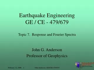
Earthquake Engineering GE / CE - 479/679 Topic 7. Response and Fourier Spectra. John G. Anderson Professor of Geophysics. F. x = y-y 0 (x is negative here). m. y. y 0. Hooke’s Law. Friction Law. c. k. z(t). Earth.

E N D
Earthquake EngineeringGE / CE - 479/679Topic 7. Response and Fourier Spectra John G. Anderson Professor of Geophysics John Anderson GE/CEE 479/679
F x = y-y0 (x is negative here) m y y0 Hooke’s Law Friction Law c k z(t) Earth John Anderson GE/CEE 479/679
In this case, the force acting on the mass due to the spring and the dashpot is the same: However, now the acceleration must be measured in an inertial reference frame, where the motion of the mass is (x(t)+z(t)). In Newton’s Second Law, this gives: or: John Anderson GE/CEE 479/679
So, the differential equation for the forced oscillator is: After dividing by m, as previously, this equation becomes: This is the differential equation that we use to characterize both seismic instruments and as a simple approximation for some structures, leading to the response spectrum. John Anderson GE/CEE 479/679
DuHammel’s Integral This integral gives a general solution for the response of the SDF oscillator. Let: The response of the oscillator to a(t) is: John Anderson GE/CEE 479/679
Let’s take the DuHammel’s integral apart to understand it. First, consider the response of the oscillator to a(t) when a(t) is an impulse at time t=0. Model this by: The result is: John Anderson GE/CEE 479/679
H(t) is the Heaviside step function. It is defined as: H(t)=0, t<0 H(t)=1, t>=0 This removes any acausal part of the solution - the oscillator starts only when the input arrives. 1 0 t=0 John Anderson GE/CEE 479/679
This is the result for an oscillator with f0= 1.0 Hz and h=0.05. It is the same as the result for the free, damped oscillator with initial conditions of zero displacement but positive velocity. John Anderson GE/CEE 479/679
The complete integral can be regarded as the result of summing the contributions from many impulses. The ground motion a(τ) can be regarded as an envelope of numerous impulses, each with its own time delay and amplitude. The delay of each impulse is τ. The argument (t- τ) in the response gives response to the impulse delayed to the proper start time. The integral sums up all the contributions. John Anderson GE/CEE 479/679
Convolutions. • In general, an integral of the form is known as a convolution. The properties of convolutions have been studied extensively by mathematicians. John Anderson GE/CEE 479/679
Examples • How do oscillators with different damping respond to the same record? • Seismologists prefer high damping, i.e. h~0.8-1.0. • Structures generally have low damping, i.e. h~0.01-0.2. John Anderson GE/CEE 479/679
Response Spectra • The response of an oscillator to an input accelerogram can be considered a simple example of the response of a structure. It is useful to be able to characterize an accelerogram by the response of many different structures with different natural frequencies. That is the purpose of the response spectra. John Anderson GE/CEE 479/679
What is a Spectrum? • A spectrum is, first of all, a function of frequency. • Second, for our purposes, it is determined from a single time series, such as a record of the ground motion. • The spectrum in general shows some frequency-dependent characteristic of the ground motion. John Anderson GE/CEE 479/679
Displacement Response Spectrum • Consider a suite of several SDF oscillators. • They all have the same damping h (e.g. h=0.05) • They each have a different natural frequency fn. • They each respond somewhat differently to the same earthquake record. • Generate the displacement response, x(t) for each. John Anderson GE/CEE 479/679
Use these calculations to form the displacement response spectrum. • Measure the maximum excursion of each oscillator from zero. • Plot that maximum excursion as a function of the natural frequency of the oscillator, fn. • One may also plot that maximum excursion as a function of the natural period of the oscillator, T0=1/f0. John Anderson GE/CEE 479/679
Definition • Displacement Response Spectrum. • Designate by SD. • SD can be a function of either frequency or period. John Anderson GE/CEE 479/679
Assymptotic properties • Follow from the equation of motion • Suppose ωn is very small --> 0. Then approximately, • So at low frequencies, x(t)=z(t), so SD is asymptotic to the peak displacement of the ground. John Anderson GE/CEE 479/679
Assymptotic properties • Follow from the equation of motion • Suppose ωn is very large. Then approximately, • So at high frequencies, SD is asymptotic to the peak acceleration of the ground divided by the angular frequency. John Anderson GE/CEE 479/679
Velocity Response Spectrum • Consider a suite of several SDF oscillators. • They all have the same damping h (e.g. h=0.05) • They each have a different natural frequency f0. • They each respond somewhat differently to the same earthquake record. • Generate the velocity response, for each. John Anderson GE/CEE 479/679
Use these calculations to form the velocity response spectrum. • Measure the maximum velocity of each oscillator. • Plot that maximum velocity as a function of the natural frequency of the oscillator, f0. • One may also plot that maximum velocity as a function of the natural period of the oscillator, T0=1/f0. John Anderson GE/CEE 479/679
Definition • Velocity Response Spectrum. • Designate by SV. • SV can be a function of either frequency or period. John Anderson GE/CEE 479/679
How is SD related to SV? • Consider first a sinusoidal function: • The velocity will be: • Seismograms and the response of structures are not perfectly sinusiodal. Nevertheless, this is a useful approximation. • We define: • And we recognize that: John Anderson GE/CEE 479/679
Definition • PSV is the Pseudo-relative velocity spectrum • The definition is: John Anderson GE/CEE 479/679
PSV plot discussion • This PSV spectrum is plotted on tripartite axes. • The axes that slope down to the right can be used to read SD directly. • The axes that slope up to the right can be used to read PSA directly. • The definition of PSA is John Anderson GE/CEE 479/679
PSV plot discussion • This PSV spectrum shows results for several different dampings all at once. • In general, for a higher damping, the spectral values decrease. John Anderson GE/CEE 479/679
PSV plot discussion • Considering the asymptotic properties of SD, you can read the peak displacement and the peak acceleration of the record directly from this plot. • Peak acceleration ~ 0.1g • Peak displacement ~ 0.03 cm John Anderson GE/CEE 479/679
Absolute Acceleration Response, SA • One more kind of response spectrum. • This one is derived from the equations of motion: • This can be rearranged as follows: • SA is the maximum acceleration of the mass in an inertial frame of reference: John Anderson GE/CEE 479/679
Summary: 5 types of response spectra • SD = Maximum relative displacement response. • SV = Maximum relative velocity response. • SA = Maximum absolute acceleration response John Anderson GE/CEE 479/679
Here are some more examples of response spectra • Magnitude dependence at fixed distance from a ground motion prediction model, aka “regression”. • Distance dependence at fixed magnitude from a ground motion prediction model, aka “regression”. • Data from Guerrero, Mexico. John Anderson GE/CEE 479/679
Data from Guerrero, Mexico, Anderson and Quaas (1988) John Anderson GE/CEE 479/679
Main Point from these spectra • Magnitude dependence. • High frequencies increase slowly with magnitude. • Low frequencies increase much faster with magnitude. John Anderson GE/CEE 479/679
Note about ground motion prediction equations • AKA “regressions • Smoother than any individual data. • Magnitude dependence may be underestimated. John Anderson GE/CEE 479/679
Note about ground motion prediction equations • Spectral amplitudes decrease with distance. • High frequencies decrease more rapidly with distance. • Low frequencies decrease less rapidly. • This feature of the distance dependence makes good physical sense. John Anderson GE/CEE 479/679