Download
1 / 31
310 likes | 429 Views
Cellular Texture Generation. We are interested in making images of surfaces covered with interacting geometry elements such as :. Scales Feathers Thorns. There are a few challenges in making images of these type :

E N D
Cellular Texture Generation
We are interested in making images of surfaces covered with interacting geometry elements such as : • Scales • Feathers • Thorns
There are a few challenges in making images of these type : • It requires a representation with more detail then texture-mapping • but are inconvenient to model with hand-crafted geometry. • It is often difficult to map appropriate texture • coordinates onto the global geometry and topology . • The placement, orientation, coloration, and shape of • the individual elements may depend on : • - neighboring elements • - surface characteristics such as local curvature . • - global phenomena such as sunlight .
Key Words – particle system , developmental models , data amplification , constraints , texture mapping , bump mapping , displacement mapping . Cellular textures are modeled by using small 3d cells constrained to lie on a surface . The cells interact to form cellular textures : surface textures with 3d geometry , orientation and color . This approach combines properties of particle systems , developmental models,and reaction diffusion methods into one system .
Development Approach For generating organic patterns it is natural to consider a biological–based simulation . biological development model is used to simulate and study patterns generated by the motions and interaction of discrete cells.
These artificial cells can move about , grow , and divide in a simulated petri dish which is called extracellular environment . The ability to form a variety of interesting patterns with the system is the reason for exploring its application to geometric texture generation . The textures modeled, are formed from many interacting geometric elements . Scales feathers or thorns can be created from a single cell , or multiple cells .
There are three main software modules : • Cellular particle simulator with surface constraints : • Automatically grow cellular textures by simulating • discrete cells on surfaces . Computes location , • orientations , sizes and other parameters of cells • based on behavioral specification. • Parameterized particle to geometry : • Converts cell position , orientations and other • parameters into shape and appearance parameters. • Render • renders the scene .
Cellular Particle Simulator • Allows the user to specify cell behaviors such as ‘go to surface’ and ‘align with neighbors’ by combining modular cell programs, which are first-order differential equation terms that modify the cell’s state . • For a particular simulation the user defines : • the cell state variables . • the extracellular environment . • the cell programs. • initial placements and other initial conditions. • The user can also stop the simulation , • change the cell programs and , restart it with the new • modifications .
Definitions A cell is an entity that has position, orientation, shape, and other parameters. It is a generalization of a particle in a particle system . Cell state variable : S = ( p , q , r , Sdie ,Ssplit , Sc0 , Sc1 , Sc2 , … , Sa0 , Sa1 , Sa2 , … ) p - position . q - orientation . r - size . Sdie - if exceeds a threshold θdie , the cell will die. Ssplit - if exceeds a threshold θsplit , the cell will split . Sci - concentrations of chemicals within the cell . Sa0 - concentrations of chemicals in the cell membrane .
Extracellular Environment Parameters which describe everything the cell can sense from its current position . Λ = (Λa0 , Λa1 , Λa2 , ··· , Λp0 , Λp0 , Λp1 , Λp1 , ··· , Λv0 , Λv1 , ··· , Λwx , Λwy , Λwz , Λu0 , Λu1 ,··· ) Λai – represent the amounts of membrane chemicals that are bound to membrane chemicals on neighboring cells. Λpi , Λpi – represents value and gradient of potential field. Λvi , Λui – other scalar and vector fields . Λwi – this vector describes the rotation that would align this cell’s ei axis with the average orientation of the adjacent cells. Example : 1 exb× exc Λwx = ∑ cos-1(exb · exc) n ||exb× exc|| b – the cell c – its neighbors c neighbors
Cell programs Each cell has several cell programs , which are first order equations describing how its state changes over time. A cell program is a function of the cell’s current state S and its environment as expressed by Λ . Different types of cells use different cell programs or different combination of the same cell program to define their behaviors . The entire system of differential equations to be solved is obtained by superposing ordinary differential equations from the cell program for every cell .
Examples of cell’s programs Go to a surface : Implements a constraint to keep a cell on the implicit surface f(x) = 0 . As the the simulation runs a cell with this program will descend the gradient and come to rest on the surface. The parameter k determines the speed with which the particle approaches the surface. P'+= -k f(p)f(p) Die if too far from surface : Will cause Sdie to rise towards the threshold quickly if the cell is greater than a certain distance d from the surface. 1 S'die+= f(p)θdie - sdie d
Align with a vector field : In this example the cell’s y-axis , ey , is alignedwith a given vector field v(x) , Which is evaluated at the cell’s current location , p . ey× v(p) v(p) wv = k cos-1(ey· ) ||ey× v(p)|| ||v(p)|| q'+= (1/2)wvq Align with neighbors : The three orientation constraints on the cell’s x y and z axes fully constrain its orientation . Constraining two axes would be sufficient in most cases . q'+= (1/2)Λwiq
Maintain unit quaternion Add a constraint to ensure that the quaternion does not stay too far from a unit quaternion during the integration of differential equations . q'+= 4k(1 – q · q)q Adhere to other cells Causes the variable sa2 (representing the surface chemical a2) to approach and stay at the value 1.0 . A pair of cells expressing a2 will stick together once they come in contact , and force is required to pull them apart . S'a2 += 1.0 – sa2
Divide until surface is covered Divide until the amount of bound surface chemical a2 reaches the level γ . Λa2 reports the total amount bound from all cells that are in contact , which gives the cell a means of determining how many neighbors it has . The value of will near one for (b >> a) and near zero for (a << b). Ssplit+= (γ, Λa2) θsplit - ssplit (a , b) (tanh((b-a) +1)/2 Set size relative to surface feature size Relates the cell size to the sizes of features in the polygon database . Achieved by providing the cells with a value Λu0 that represents the area of the nearest triangle . Could also be used to capture surface curvature . r'+=Λu0 - r
Example of reaction-diffusion in discrete cells The full derivation of this set of equations is beyond the scope of this presentation . Sc0 is the activator and sa1 is the inhibitor , which is propagated by the activity of membrane chemicals . 2 2 s'c0+= -20Λa0 /Λa2 + 10sc0/(1 + sc0 ) – 0.5 sc0 +13 Defines a generic switch that tends to drive sc0 towards one of two values , depending on the influence of the term Λa0 /Λa2 . s'a1+= 0.95Λa0 /Λa2 } Determine interactions of membrane chemicals that lead to an effective diffusion of the value of sa1 among the cells .the value sc0 can then be used to determine the final rendered shape of the cell . s'a1+=(3,sc0)sc0 s'a0+= 5 – sa0 s'a1+=-sa1 s'a2+= 1 – sa2
Surface constraints • There are several types of surface classes : • polygonal mesh surfaces . • Implicit function surfaces . • isosurfaces of volume data surfaces. The surface constraint cell program, evaluates an implicit function to enable the cell to find and stay on the surface. Because the surface could be a mesh, a rough approximation to an implicit function is created for these meshes . Any implicitization method will work , and in fact it doesn’t have to be very exact . We implement this function by constructing an approximate kd-tree for the triangular mesh .
Particle converter • Converts information about the particles and their • environment into geometry and appearance parameters for • rendering . • It enables us to do a variety of useful operations : • Choosing an appropriate • representation for each cell • based on its screen size . • as you can see in the picture • the thorny spheres at further • distance are rendered with • fewer polygons.
2. smoothly changing the appearance of a cell based on continuously varying parameters.
3. using the cell position to generate spatial subdivision . 4. using the cell orientation to compute a flow on the surface . 5. experimenting with various colorations and geometries using the same simulation dataset .
Scales • cell program used: • Divide until the surface is covered • Stay on the surface • Die if pushed to far from the surface. • Soft constraint to align y-axes with the gradient of the • surface implicit function • Align there x and z axes with their neighbors .
A knotty problem Capable of creating textures for surfaces with unusual topologies.
Thorny head ( the first pic ) Main point - Changing cell size to match surface features . If you look closely you can see there is a finer texture and geometry around the eyes and mouth . The cell size is related to the detail level in the underlying polygonal model. Thorny spheres • Several important capabilities : • the creation of a simple reaction-diffusion patterns on a • surface . • the use of the concentrations of cell chemicals to change • parameters of the rendered geometry . • the ability to restart simulations from an previous state with • new cell programs , causing new behaviors to occur .
A bear of a surface • A fur-covered model of a bear defined as an isosurface of • sampled volume data . • The bear on the left , started from a single cell and used a • set of rules similar to the rules used in the scales picture . • The bear on the right started from about 2000 cells , • each cell choused one neighbor to align with , and cells • didn’t try to align with neighbors that were oriented in the • directly opposing direction .
conclusion The combination of particle system constraint techniques with developmental models enables the generation of a variety of cellular textures as shown in the figures . Some difficulties: Shapes : the particle converter might make objects with undesirable intersections . This can be minimized by a careful choice of cell geometry . A more robust solution is to use the desired geometric shape directly in the cellular particle simulation .
Experience with writing cell programs : Writing cell programs can be difficult, it Requires a Different intuition than other types of programming , and often takes a while to get right . (gets easier with practice) . Simulation speed : Can be very slow (many hours) for some kinds of cell programs , or very fast (a few seconds) for others. Generally , performance degrades as the differential equations get stiff . Data explosion : The data produced both by the simulation and by the particle converter can get very large .
Future work • continue extending and refining the cell programs to generate • more complex cellular textures . • running simulations on objects as they move and change shape . • modeling the motion of feathers on the wings of a flying bird . • implementing more sophisticated cell geometries in the particle • simulator in order to generate more realistic placement of detail • and avoid self-intersections in the rendering . • explore the possibilities of creating shapes directly from the • fundamental interactions of the cells , without the surface • constraint .
Bibliography • Computer Graphics Proceedings , Annual Conference • Series 1995