Download
1 / 18
190 likes | 451 Views
Social Network Analysis in R. Elijah Wright IV Lab meeting, 3-31-2004 [Based on Carter Butts’ SNA tutorial]. Loading up SNA…. #Load the mva (multivariate analysis) library library(mva) #Load the SNA library by Carter Butts of UCI library(sna). What kind of data does it expect?.

E N D
Social Network Analysis in R Elijah Wright IV Lab meeting, 3-31-2004 [Based on Carter Butts’ SNA tutorial]
Loading up SNA… • #Load the mva (multivariate analysis) library • library(mva) • #Load the SNA library by Carter Butts of UCI • library(sna)
What kind of data does it expect? • Most of the SNA routines expect either raw square matrices or m*n*n arrays – where n*n are the rows and columns, and m is the index of the graph stack. This lets you operate on stacks of matrices (and so stacks of graphs) rather than simple graphs. • In other words, this thing does a lot of very complicated things to make hard things easier and the impossible – possible. • Either directed or undirected graphs – if it matters, the function will have an extra parameter inside it to control results.
Some R stuff for people who don’t use it… • R is pretty friendly – you can examine the guts of the functions you’re using to get a grip on what they do. • How – simply type the name of the function and press enter – you get a dump of the code to the screen. Same goes for variables and data structures. • If you need a summary of some thing, do summary(variable)
First, to generate some random social network data • To begin, let us imagine that we are assessing a population of 25 actors, each of whom may have either a weak, moderate, or strong tendency to send or recieve network ties. To model this tendency, we assign each actor randomly to one of the nine possible states and draw from two binomial distributions as follows: • #Create a vector of incoming tie parameters for social support • sup.in<-rbinom(25,50,sample(c(0.1,0.5,0.9),25,replace=TRUE)) • #Create a vector of outgoing tie parameters for social support • sup.out<-rbinom(25,50,sample(c(0.1,0.5,0.9),25,replace=TRUE)) • Each actor, then, has two "parameters," one reflecting a tendency to receive ties, and another to send them. • [look at sup.in and sup.out]
Buildin’ a matrix • #Draw a matrix of tie probabilities for social support • sup.tp<-matrix(nrow=25,ncol=25) • for(i in 1:25) • for(j in 1:25) • sup.tp[i,j]<-rbeta(1,sup.out[i]+sup.in[j]+1,100-(sup.out[i]+sup.in[j])+1) • #Model tie probs as betas (this makes bayesian network analysis a bit easier…)
Building the random graph… • #Draw the social support graph, using the tie probabilities • support<-rgraph(25,tprob=sup.tp) • (Now, to this point, everything we’ve used is in the R base – rgraph is the first function we’ve seen that’s sourced from the SNA package. • Look at rgraph…. • Given the above parameters, rgraph produces a 25-actor random digraphic adjacency matrix with a zero-valued diagonal, using the tie probabilities given by the sup.tp matrix. If we were so inclined, we could set other options in the above command to draw multiple matrices using the same tie probabilities, to permit values on the diagonal, or to force the matrix to be symmetric (for simple graphs). At the moment, however, we shall keep our support network in its present form, and continue with our example.
Some miscellany from Butts’ tutorial – this at least gets us some interesting transformations of the data • Having produced a support network, we now consider some fictitious mental health outcomes associated with it. In each of the cases below, we use the rnorm function to create 25 draws from a normal distribution with mean equal to a function of one or more nodal indices. Later, we shall examine the use of these nodel index functions more closely; for now, simply recognize that we can use properties of individual positions to more or less seamlessly create a set of associated variables for subsequent analysis. • Run ?rnorm • #Now for some fictitious mental health outcomes.... • sup.outc.1<-rnorm(25,degree(support,cmode="indegree"),2) • sup.outc.2<-rnorm(25,stresscent(support),2) • sup.outc.3<-rnorm(25,degree(support,cmode="outdegree")-degree(support,cmode="indegree"),1) • sup.outc.4<-rnorm(25,0,10)
Friendship and Advice networks… • #Draw a symmetric friendship network • friends<-rgraph(15,tprob=0.3,mode="graph") • (The rgraph routine is fairly intelligent about interpreting the tprob argument; it is used as an overall tie probability, a per-matrix tie probability, or a per-tie tie probability, when given as a single number, a vector, or a matrix, respectively.) The mode parameter here tells rgraph to draw a simple graph (that is, a symmetric adjacency matrix) instead of a digraph (which is the default option). Compare this with a simulated "advice" relation: • #Draw an unrelated advice network (asymmetric!) • advice<-rgraph(15,tprob=0.2)
Authority network • #Draw yet another network, calling it authority. We'll make it into a hierarchy.... • authority<-rgraph(15,tprob=0.3) • authority[lower.tri(authority)]<-0 • #Zero out the lower triangle
Prestige network • A fictitious "prestige" relation which depends upon both advice and friendship in a reasonably intuitive fashion. We proceed by creating a matrix of tie probabilities which will then be used with rgraph() to draw the actual network. Unlike our previous example, however, we here use a logistic density to determine the tie probabilities: • #Draw a prestige network which depends upon the first two relations, but not the third • pres.tp<-matrix(nrow=15,ncol=15) • for(i in 1:15) • for(j in 1:15) • pres.tp[i,j]<-plogis(2*friends[i,j]*advice[j,i]+5*advice[j,i]-3*friends[i,j]-2*advice[i,j]) • prestige<-rgraph(15,m=1,tprob=pres.tp)
Sociometric Power Graph • #Draw a sociometric power graph which is based on the second and third relations, but not the first • perpower <-matrix(rnorm(15^2,2*as.vector(advice)+5*as.vector(authority),3),nrow=15,ncol=15) • Here, we model the ties of the former as being iid normal, with means dependent upon the states of the latter relations. This is accomplished via rnorm, using the following command:
Building a graph stack • #For convenience, stick our relations into one stack • rrel<-array(dim=c(5,15,15)) • rrel[1,,]<-friends • rrel[2,,]<-advice • rrel[3,,]<-prestige • rrel[4,,]<-authority • rrel[5,,]<-perpower • rrel.names<-c("friends","advice","prestige","authority","perpower")
A star, a tree, and a clique • #Enter three archetypal structures • team.arch<-array(dim=c(3,7,7)) • team.arch[1,,]<-t(matrix(c( • 0,1,1,1,1,1,1, • 1,0,0,0,0,0,0, • 1,0,0,0,0,0,0, • 1,0,0,0,0,0,0, • 1,0,0,0,0,0,0, • 1,0,0,0,0,0,0, • 1,0,0,0,0,0,0),nrow=7,ncol=7)) • team.arch[2,,]<-t(matrix(c( • 0,1,1,0,0,0,0, • 0,0,0,1,1,0,0, • 0,0,0,0,0,1,1, • 0,0,0,0,0,0,0, • 0,0,0,0,0,0,0, • 0,0,0,0,0,0,0, • 0,0,0,0,0,0,0),nrow=7,ncol=7)) • team.arch[3,,]<-t(matrix(c( • 0,1,1,1,1,1,1, • 1,0,1,1,1,1,1, • 1,1,0,1,1,1,1, • 1,1,1,0,1,1,1, • 1,1,1,1,0,1,1, • 1,1,1,1,1,0,1, • 1,1,1,1,1,1,0),nrow=7,ncol=7))
Some other stuff you can do… • Betweenness centrality: • betweenness(graph) • Geodesic distances and shortest path: • geodist(graph) • Centralgraph – finds the central graph of a graph stack. • Graph density – gden(graph) • Rmperm – randomly permute the rows and columns of a graph stack • Upper.tri.remove – well, you can guess what this does. • Diag.remove – Ha. Converts diagonals to “not applicable” values.
More stuff ---- • Correlations and regression models as applied to graphs • Plots, multidimensional scaling (MDS) at the drop of a hat…. • Gplot(), cmdscale()
A little Tulip stuff (and a demo) at the end … • Tulip – large-scale graph network visualization tool • Can do 500k nodes on a PIII/600 w/256MB of memory (this is freaking awesome compared to anything else I’ve seen!) • OpenGl, C, yay! • It can import matrices, graphml format, random graphs, its own format, et cetera et cetera. Pretty cool. Does clustering and various layouts (spring, Fruchterman-Rheingold, cones, tree layouts) internally. • Problems I observe so far – pretty easy to generate random graphs in it, but pretty hard to get edges to show up in them Importing a graphml file gets you a display with sensible edges… i guess we probably need some converters to get data into an ‘attractive’ format like what we have for Pajek currently. • Not quite the same uses as Pajek, but it is nice to be able to do freakishly huge graphs and actually get a display.
The End • This is the end This is the end This is the end This is the end This is the end This is the end This is the end This is the end This is the end This is the end This is the end This is the end This is the end This is the end This is the end This is the end This is the end This is the end This is the end This is the end This is the end This is the end This is the end This is the end This is the end This is the end This is the end This is the end This is the end