Download
1 / 80
810 likes | 830 Views
Explore CT equipment, basic physical principles, radiation protection rules, dosimetry quantitites, and more at the National Turkish Medical Physics Congress. Learn about the history and advancements of CT technology from a renowned physicist.

E N D
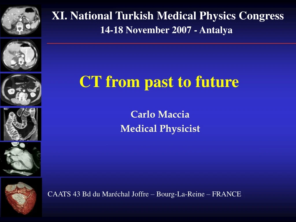
XI. National Turkish Medical Physics Congress 14-18 November 2007 - Antalya CT from past to future Carlo Maccia Medical Physicist CAATS 43 Bd du Maréchal Joffre – Bourg-La-Reine – FRANCE
Content • CT equipment and technology • Recall of basic physical principles of CT • Radiation protection rules and QC • CT dosimetry quantities • Reference Dose values and Quality criteria for CT images
INTRODUCTION Computed tomography (CT) was commercially introduced into radiology in 1972 and was the first fully digital imaging device making it truly revolutionary in diagnostic imaging. In 1979, Godfrey Hounsfield and Allen Cormack were awarded the Nobel Prize in Physiology and Medicine for their contributions in the development of CT. CT differs from conventional projection imaging in two significant ways: • CT forms a cross-sectional tomographic image, eliminating the superimposition of structures that occur in plane film imaging because of the compression of three-dimensional body structures into the two-dimensional recording system • the sensitivity of CT to subtle differences in x-ray attenuation is at least a factor of 10 higher than normally achieved by film-screen recording systems
THE BASIC PHYSICS PROBLEM Under ideal conditions (monochromatic beam, ideal collimation, perfect detection, etc) x-ray intensity observes an exponential decay law: N = N0 e-x where N0 and N are the intensities of the incident and exiting x-rays, respectively,x is the path length through the attenuating material, and is the linear attenuation coefficient of the material along the path x. ASIDE If we had a block consisting of a single attenuating material with unknown , we could measure its length (x) and the incident (N0) and exiting intensities (N) , and then solve for .
So essentially we have Now suppose we have an object with unknown contents, we can make a measurement of x-ray attenuation along a straight line through it but for all intense of purposes all that this will tell us is a single number representing the total attenuation of the material in the path. What we really want is the attenuation coefficient at each position along the path.
Consider the case for n = 4 and each block had a size x: We can see from the above illustration that in order to solve for 1, 2, 3 and 4, we would need 4 independent equations (N1, N2, N3 and N4). and thus With a single transmission measurement, the separate attenuation coefficients cannot be determined because there are too many unknown values of i where i = 1,2,3 ,…, n. In order to solve this equation for the n values of i we will need n2 independent transmission equations (the above equation would be one of the n2required equations).
DATA ACQUISITION GEOMETRIES A variety of geometry's have been developed to acquire the x-ray transmission data needed for image reconstruction in CT. Some geometry's have been tagged as a “generation” of CT scanner and these labels are useful in different scanner designs. The following scanner geometry's, data acquisition modes and primary technologies have been used to date: • First Generation CT Scanner (EMI, 1973) • Second Generation CT Scanner (1974) • Third Generation CT Scanner (GE & Siemens, 1975-76) • Fourth Generation CT Scanner (1977) • Low Voltage Slip Ring Technology (Siemens, 1982) • Fifth Generation CT Scanner (1984) • Spiral CT Scanner (Siemens, 1988) • Multi-slice CT Scanner (Dual-slice, Elscint, 1992) • Multi-slice CT Scanner (Quad-slice, 1998) • Dual source CT (64-slice with two X-ray tubes, Philips 2006, 256-slice Toshiba)
FIRST GENERATION CT SCANNER (Translate/Rotate) First Head Scanner
NOTE • this method was theoretically immune to the effects of scattered x-ray (single • detector system) • because of the long scan times, this method of scanning was applicable to scanning • of parts of anatomy that could have been kept motionless, such as the head
THIRD GENERATION CT SCANNER (Rotate/Rotate) Predominant design of current commercially available CT scanners
LOW VOLTAGE SLIP RING TECHNOLOGY Some third and fourth generation CT scanners employ a slip ring to supply power and receive signals from rotating parts. In the slip-ring method, an electrical conductive brush moves along a ring-shaped electrically conductive rail. The use of a slip ring permits high-speed continuous scanning, and dramatically increases both the performance and range of clinical applications of CT scanning. • allows for 1 second ( or < 1 second or sub-second) scan times • allows for helical (or volumetric) scanning
A look inside a rotate/rotate CT Detector Array and Collimator X-Ray Tube
A Look Inside a Slip Ring CT Note: how most of the electronics is placed on the rotating gantry X-Ray Tube Detector Array Slip Ring
SPIRAL CT SCANNERS (Helical Scanning Mode) • If the x-ray tube can rotate constantly, the patient can then be moved continuously through the beam, making the examination much faster
MULTI-SLICE CT SCANNERS (Quad Slice) To build quad-slice spiral CT scanners, manufacturers had to develop detector arcs with more than four elements in the longitudinal (z) axis direction, creating a curved two-dimensional detector arrays. GE Scanners
Fast + Poor Image quality Fast + Improved Image quality Dual Source CT Single source CT
AXIAL IMAGE RECONSTRUCTION The task of reconstruction is to compute an attenuation coefficient for each picture element (pixel) and then to assign a CT number to each of these elements. • in order to create multiple projections in a single 360° • tube rotation, during a single projection the x-ray tube • is pulsed and the detector array is sampled after each • pulse
A B IMAGE RAY SUM • For a single detector, a ray sum consists of all the linear attenuation coefficient data • along the corresponding x-ray beam path (eg: path AB) • For a single x-ray beam path, the ray sum is not the simple summation of the • attenuation coefficients of the intercepted pixels.
I0 In Pixel Position Output Intensity I1 = I0 e-1w 1 I2 = I1 e-2w = I0e-w(1 + 2) 2 n In = I0e-w(1 + 2 + … + n) 1 + 2 + 3 + … + n = 1 ln (I0/ In) w Recall from previous lecture notes therefore Ray Sum Value Actually, the ray sum value that is computed is proportional to the sum of the n attenuation coefficients along the x-ray beam path
IMAGE PROJECTION DetectorPosition • a projection is defined as the set of ray sums measured in all detectors during a • single x-ray tube pulse • typically anywhere between 800 - 1000 projections are collected in one 360° tube • rotation to reconstruct a singleaxial image
Images slices are reconstructed into a matrix consisting of multiple volume elements (voxel) each with a unique value.
IMAGE INTERPOLATION (SPIRAL CT) PROBLEM The volume scanned in a single rotation differs between the conventional and helical scanning methods. ANSWER Interpolate desired axial image from volume data set prior to image reconstruction.
New CT Features • The new helical scanning CT units allow a range of new features, such as : • CT fluoroscopy, where the patient is stationary, but the tube continues to rotate • multislice CT, where up to 64 (128 - 256) slices can be collected simultaneously • 3-dimensional CT and CT endoscopy • Cardiac image acquisition during relevant heart phases (ECG pulsing synchronization)
CT Fluoroscopy • Real Time Guidance(up to 8 fps) • Great Image Quality • Low Risk • Faster Procedures (up to 66% fasterthan non fluoroscopicprocedures) • Approx. 80 kVp, 30 mA
Content • CT equipment and technology • Recall of basic physical principles of CT • Radiation protection rules and QC • CT dosimetry quantities • Reference Dose values and Quality criteria for CT images
CT NUMBER CT Number = 1000 p - w = Hounsfield Unit (HU) w The final result of the CT image reconstruction is an accurate estimate of the x-ray absorption values characteristic of individual voxels. where p is the linear attenuation value assigned to a given pixel and w is the linear attenuation value of water. • ASIDE • wis obtained during calibration of the CT scanner • by definition, the HU of water is 0 and the HU value for air is -1,000 • above equation defines 100 HU as equal to a 10 % difference in the linear • attenuation coefficient relative to water • the value 1000 in the numerator is a scale factor and determines the contrast scale
FIELD-OF-VIEW (FOV) FOV is the diameter of the area being imaged (e.g: 25 cm Head and 35 cm Body scan) • CT pixel size is determined by dividing the FOV by the matrix size (typically • 512 x 512 – 768 x 768 or 1024 x 1024)
IMAGE DISPLAY • reconstructed images are viewed on a CRT monitor or printed onto film using a laser printer • each pixel is normally represented by 12 bits, or 4096 gray levels, which is larger than the display range of monitors or film • window width and level are used to optimize the appearance of CT images by • determining the contrast and brightness levels assigned to the CT image data
IMAGE QUALITY Image quality may be characterized in terms of: • contrast • noise • spatial resolution • ASIDE • in general, image quality involves tradeoffs between these three factors and patient • dose. • artifacts encountered during CT scanning can degrade image quality
IMAGE CONTRAST CT contrast is the difference in the HU values between tissues. This contrast generally increases as kVp decreases but is not affected by mAs or scan time. CT Photon Energy Range (120 or 140 kVp) • CT contrast may be artificially increased by adding a contrast medium such as • iodine • image noise may prevent detection of low-contrast objects such as tumors with a • density close to the adjacent tissue • the displayed image contrast is primarily determined by the CT window width and • window level settings.
LOW CONTRAST RESOLUTION • Measurement Technique Catphan 500 (phantom) Insert Diametre : 2 mm to 15 mm. Contrast levels : 0.3, 0.5 and 1% Supra slice (Periphery) Z = 40 mm Subs slice (centre) Z= 3, 5, 7 mm 1% 0,5% 0,3%
IMAGE NOISE • The sources of image noise in CT are: • quantum mottle (the number of photons used to make an image) • inaccuracies in the image reconstruction process (software filter phase); and • electronic noise introduced after detection • Noise in CT is usually defined as the standard deviation () of the CT numbers • calculated from pixel values in a predefined region-of-interest (ROI) using an image • of a uniform material (usually water). The selected ROI region should be void of • objects and cover a sufficiently large image area (circular diameter > 10 mm). • For GE scanners: • ROI CT number Average Value = 0.0 3.0 HU • ROI CT number Standard Deviation = 3.5 0.7 HU
ROI Area = 13.17 cm2 Mean = 1.75 Std. Dev. = 2.9 NOTE: Noise = 2.9 Scan Parameters: Small Scan FOV, 25 cm DFOV, 5122 Matrix, Standard Resolution, Peristaltic Option OFF, 13.17 cm2 CROI, Normal Scan Type, 5 mm slice thickness, 170 mA and 2 sec scan time
ELECTRONIC NOISE • in modern CT scanners electronic noise is kept to a minimum • a CT scanner whose noise is dominated by the detection of a finite number of x-rays • (quantum mottle) is called quantum limited • in a quantum limited CT scanner • (noise)2 1 • patient dose • a CT scanner can be shown to be quantum limited by plotting • (noise)2 vs 1 • (any parameter that affects patient dose) • and determining the magnitude of the y-intercept of the interpolated linear curve fit
Since in a quantum limited CT scanner • (noise)2 1 • patient dose/pixel • then • (noise)2 1 • B • D • H • w3 • where • B - is the fractional transmission of the patient • D - is the maximum surface dose ( mAs) • H - is the slice thickness • w - is the reconstructed pixel width • quantum mottle (and thus noise) decreases as the number of photons increases • CT noise is generally reduced by increasing the kVp, mA or scan time (if all other parameters are kept constant) • CT noise is also reduced by increasing voxel size (ie: by decreasing matrix size, increasing FOV or increasing the slice thickness) • typically noise with a modern CT scanner system is approximately 5 HU (or • 0.5% difference in attenuation coefficient)
IMAGE RESOLUTION • Spatial resolution is the ability to discriminate between adjacent objects and is a • function of pixel size. • If the CT FOV is D and the matrix size is M, then pixel size is D/M. • Example: • For a typical head scan with a FOV of 25 cm and a matrix of 512 pixels, the pixel size is 0.5 mm • Because two pixels are required to define a line pair (lp), the best achievable spatial resolution is 1 lp/mm • typically resolution in CT scanning ranges from 0.5 to 1.5 lp/mm • the axial resolution may be improved by operating in a high resolution mode using a smaller FOV or a larger matrix size • factors that may also improve CT spatial resolution by reducing image blur include • smaller focal spots, smaller detectors and more projections • resolution perpendicular to the section is dependent on slice thickness and is important in Sagittal and Coronal image reconstruction
IMAGE RESOLUTION • Measurement Technique • MTF (Modulation Transfer Function) objective method • Assessment of a bar pattern – subjective method
IMAGE RESOLUTION • MTF can be considered as a reliable measure of the information transfer from the object to the image. It illustrates, for each individual spatial frequency, the progressive degradation of the signal due to the system in terms of % of contrast loss.
IMAGE RESOLUTION • The MTF is assessed from the Fourier Transform of the Linear Spread Function (LSF) which is a measure of the ability of a system to form sharp images; it is determined by measuring the spatial density distribution on film of the X-ray image of a narrow slit in a dense metal, such as lead. • The point spread function (PSF) describes the response of an imaging system to a point source or point object
IMAGE RESOLUTION The image of the « point object » is not a single point but a set of different points representing the degradation of the signal.
IMAGE RESOLUTION • MTF curves at 50 %, 10 % and 2 %. PQ 5000
IMAGE RESOLUTION • Typical values • Standard mode : 7 line pairs / cm . • Maximum values : 17 to 18 line pairs / cm(high resolution mode)
IMAGE RESOLUTION (influencing factors) • Acquisition • Number of projections