Download
1 / 105
1.07k likes | 1.1k Views
Explore efficient and reliable packet routing in network switches and routers, covering loop-free routes, routing algorithms, creating routing tables, and specialized routing techniques like flooding and deflection.

E N D
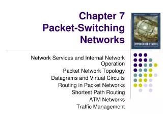
Packet-Switching Networks Routing in Packet Networks
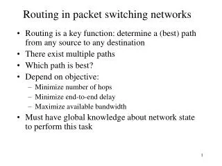
1 3 6 4 2 Node (switch or router) 5 Routing in Packet Networks • Three possible (loopfree) routes from 1 to 6: • 1-3-6, 1-4-5-6, 1-2-5-6 • Which is “best”? • Min delay? Min hop? Max bandwidth? Min cost? Max reliability?
Creating the Routing Tables • Need information on state of links • Link up/down; congested; delay or other metrics • Need to distribute link state information using a routing protocol • What information is exchanged? How often? • Exchange with neighbors; Broadcast or flood • Need to compute routes based on information • Single metric; multiple metrics • Single route; alternate routes
Routing Algorithm Requirements • Responsiveness to changes • Topology or bandwidth changes, congestion • Rapid convergence of routers to consistent set of routes • Freedom from persistent loops • Optimality • Resource utilization, path length • Robustness • Continues working under high load, congestion, faults, equipment failures, incorrect implementations • Simplicity • Efficient software implementation, reasonable processing load
2 7 1 8 B 1 3 3 A 6 5 1 5 4 2 VCI 4 Host Switch or router 3 5 2 5 C 6 D 2 Routing in Virtual-Circuit Packet Networks • Route determined during connection setup • Tables in switches implement forwarding that realizes selected route
Node 3 Incoming Outgoing Node 6 Node 1 Node VCI Node VCI 1 2 6 7 Incoming Outgoing Incoming Outgoing 1 3 4 4 Node VCI Node VCI Node VCI Node VCI 4 2 6 1 3 7 B 8 A 1 3 2 6 7 1 2 3 1 B 5 A 5 3 3 6 1 4 2 B 5 3 1 3 2 A 1 4 4 1 3 B 8 3 7 3 3 A 5 Node 4 Incoming Outgoing Node VCI Node VCI 2 3 3 2 Node 2 Node 5 3 4 5 5 Incoming Outgoing Incoming Outgoing 3 2 2 3 Node VCI Node VCI Node VCI Node VCI 5 5 3 4 C 6 4 3 4 5 D 2 4 3 C 6 D 2 4 5 Routing Tables in VC Packet Networks • Example: VCI from A to D • From A & VCI 5 → 3 & VCI 3 → 4 & VCI 4 • → 5 & VCI 5 → D & VCI 2
Node 3 Destination Next node Node 6 Node 1 1 1 Destination Next node Destination Next node 2 4 1 3 2 2 4 4 2 5 3 3 5 6 3 3 4 4 6 6 4 3 5 2 5 5 6 3 Node 4 Destination Next node 1 1 2 2 Node 2 Node 5 3 3 Destination Next node Destination Next node 5 5 1 1 1 4 6 3 3 1 2 2 4 4 3 4 5 5 4 4 6 5 6 6 Routing Tables in Datagram Packet Networks
0001 0100 1011 1110 0000 0111 1010 1101 1 4 3 R2 R1 5 2 0011 0101 1000 1111 0011 0110 1001 1100 0001 4 0100 4 1011 4 … … 0000 1 0111 1 1010 1 … … Non-Hierarchical Addresses and Routing • No relationship between addresses & routing proximity • Routing tables require 16 entries each
0100 0101 0110 0111 0000 0001 0010 0011 1 4 3 R2 R1 5 2 1100 1101 1110 1111 1000 1001 1010 1011 00 1 01 3 10 2 11 3 00 3 01 4 10 3 11 5 Hierarchical Addresses and Routing • Prefix indicates network where host is attached • Routing tables require 4 entries each
Specialized Routing • Flooding • Useful in starting up network • Useful in propagating information to all nodes • Deflection Routing • Fixed, preset routing procedure • No route synthesis
Flooding Send a packet to all nodes in a network • No routing tables available • Need to broadcast packet to all nodes (e.g. to propagate link state information) Approach • Send packet on all ports except one where it arrived • Exponential growth in packet transmissions
1 3 6 4 2 5 Flooding is initiated from Node 1: Hop 1 transmissions
1 3 6 4 2 5 Flooding is initiated from Node 1: Hop 2 transmissions
1 3 6 4 2 5 Flooding is initiated from Node 1: Hop 3 transmissions
Limited Flooding • Time-to-Live field in each packet limits number of hops to certain diameter • Each switch adds its ID before flooding; discards repeats • Source puts sequence number in each packet; switches records source address and sequence number and discards repeats
Deflection Routing • Network nodes forward packets to preferred port • If preferred port busy, deflect packet to another port • Works well with regular topologies • Manhattan street network • Rectangular array of nodes • Nodes designated (i,j) • Rows alternate as one-way streets • Columns alternate as one-way avenues • Bufferless operation is possible • Proposed for optical packet networks • All-optical buffering currently not viable
0,0 0,1 0,2 0,3 1,0 1,1 1,2 1,3 2,0 2,1 2,2 2,3 3,0 3,1 3,2 3,3 Tunnel from last column to first column or vice versa
busy Example: Node (0,2)→(1,0) 0,0 0,1 0,2 0,3 1,0 1,1 1,2 1,3 2,0 2,1 2,2 2,3 3,0 3,1 3,2 3,3
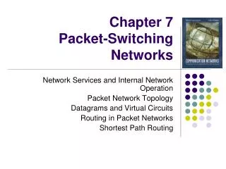
Chapter 7Packet-Switching Networks Shortest Path Routing
Shortest Paths & Routing • Many possible paths connect any given source and to any given destination • Routing involves the selection of the path to be used to accomplish a given transfer • Typically it is possible to attach a cost or distance to a link connecting two nodes • Routing can then be posed as a shortest path problem
Routing Metrics Means for measuring desirability of a path • Path Length = sum of costs or distances • Possible metrics • Hop count: rough measure of resources used • Reliability: link availability; BER • Delay: sum of delays along path; complex & dynamic • Bandwidth: “available capacity” in a path • Load: Link & router utilization along path • Cost: $$$
Shortest Path Approaches Distance Vector Protocols • Neighbors exchange list of distances to destinations • Best next-hop determined for each destination • Ford-Fulkerson (distributed) shortest path algorithm Link State Protocols • Link state information flooded to all routers • Routers have complete topology information • Shortest path (& hence next hop) calculated • Dijkstra (centralized) shortest path algorithm
Distance VectorDo you know the way to San Jose? San Jose 294 San Jose 392 San Jose 596 San Jose 250
Local Signpost Direction Distance Routing Table For each destination list: Next Node Distance Table Synthesis Neighbors exchange table entries Determine current best next hop Inform neighbors Periodically After changes dest next dist Distance Vector
j i Shortest Path to SJ Focus on how nodes find their shortest path to a given destination node, i.e. SJ San Jose Dj Cij Di If Diis the shortest distance to SJ from i and if j is a neighbor on the shortest path, then Di = Cij + Dj
San Jose j' j i j" But we don’t know the shortest paths i only has local info from neighbors Dj' Cij' Dj Cij Pick current shortest path Cij” Di Dj"
SJ sends accurate info San Jose Accurate info about SJ ripples across network, Shortest Path Converges Why Distance Vector Works 1 Hop From SJ 2 Hops From SJ 3 Hops From SJ Hop-1 nodes calculate current (next hop, dist), & send to neighbors
Bellman-Ford Algorithm • Consider computations for one destination d • Initialization • Each node table has 1 row for destination d • Distance of node d to itself is zero: Dd=0 • Distance of other node j to d is infinite: Dj=, for j d • Next hop node nj = -1 to indicate not yet defined for j d • Send Step • Send new distance vector to immediate neighbors across local link • Receive Step • At node j, find the next hop that gives the minimum distance to d, • Minj { Cij + Dj } • Replace old (nj, Dj(d)) by new (nj*, Dj*(d)) if new next node or distance • Go to send step
Bellman-Ford Algorithm • Now consider parallel computations for all destinations d • Initialization • Each node has 1 row for each destination d • Distance of node d to itself is zero: Dd(d)=0 • Distance of other node j to d is infinite: Dj(d)= ,for j d • Next node nj = -1 since not yet defined • Send Step • Send new distance vector to immediate neighbors across local link • Receive Step • For each destination d, find the next hop that gives the minimum distance to d, • Minj { Cij+ Dj(d) } • Replace old (nj, Di(d)) by new (nj*, Dj*(d)) if new next node or distance found • Go to send step
2 3 1 1 5 2 4 6 3 1 3 2 2 5 4 Table entry @ node 3 for dest SJ Table entry @ node 1 for dest SJ San Jose
D3=D6+1 n3=6 D6=0 2 3 1 1 5 2 4 6 3 1 3 2 2 5 4 D6=0 D5=D6+2 n5=6 1 0 San Jose 2
2 3 1 1 5 2 4 6 3 1 3 2 2 5 4 3 1 3 0 San Jose 6 2
2 3 1 1 5 2 4 6 3 1 3 2 2 5 4 1 3 3 0 San Jose 6 4 2
2 3 1 1 5 2 4 6 3 1 3 2 2 5 4 1 5 3 3 0 San Jose 4 2 Network disconnected; Loop created between nodes 3 and 4
2 3 1 1 5 2 4 6 3 1 3 2 2 5 4 5 7 3 5 3 0 San Jose 2 4 Node 4 could have chosen 2 as next node because of tie
2 3 1 1 5 2 4 6 3 1 3 2 2 5 4 7 5 7 0 5 San Jose 2 4 6 Node 2 could have chosen 5 as next node because of tie
2 3 1 1 5 2 4 6 3 1 3 2 2 5 4 7 7 9 5 0 San Jose 6 2 Node 1 could have chose 3 as next node because of tie
(a) 1 2 3 4 1 1 1 (b) 1 2 3 4 X 1 1 Counting to Infinity Problem Nodes believe best path is through each other (Destination is node 4)
Problem: Bad News Travels Slowly Remedies • Split Horizon • Do not report route to a destination to the neighbor from which route was learned • Poisoned Reverse • Report route to a destination to the neighbor from which route was learned, but with infinite distance • Breaks erroneous direct loops immediately • Does not work on some indirect loops
(a) 1 2 3 4 1 1 1 (b) 1 2 3 4 X 1 1 Split Horizon with Poison Reverse Nodes believe best path is through each other
Link-State Algorithm • Basic idea: two step procedure • Each source node gets a map of all nodes and link metrics (link state) of the entire network • Find the shortest path on the map from the source node to all destination nodes • Broadcast of link-state information • Every node i in the network broadcasts to every other node in the network: • ID’s of its neighbors: Ni=set of neighbors of i • Distances to its neighbors: {Cij | j Ni} • Flooding is a popular method of broadcasting packets
w' x' z' w' w x x z s w" w" Dijkstra Algorithm: Finding shortest paths in order Find shortest paths from source s to all other destinations Closest node to s is 1 hop away 2nd closest node to s is 1 hop away from s or w” 3rd closest node to s is 1 hop away from s, w”, or x
Dijkstra’s algorithm • N: set of nodes for which shortest path already found • Initialization: (Start with source node s) • N = {s}, Ds = 0, “s is distance zero from itself” • Dj=Csj for all j s, distances of directly-connected neighbors • Step A: (Find next closest node i) • Find i N such that • Di = min Dj for j N • Add i to N • If N contains all the nodes, stop • Step B: (update minimum costs) • For each node j N • Dj = min (Dj, Di+Cij) • Go to Step A Minimum distance from s to j through node i in N
2 1 3 1 2 1 1 5 2 5 3 2 3 2 1 2 1 3 3 3 3 3 3 3 1 3 1 2 6 6 6 6 6 6 6 3 5 2 4 3 4 4 4 4 4 4 4 4 1 2 3 2 2 1 2 2 2 2 2 2 2 1 3 3 1 1 5 5 5 5 5 5 5 4 5 5 2 2 3 3 1 2 1 2 3 3 4 4 2 2 1 3 1 1 3 1 5 5 2 2 3 3 1 2 1 2 3 3 4 4 Execution of Dijkstra’s algorithm
2 1 3 1 2 1 1 5 2 5 3 2 3 1 2 3 3 3 3 3 3 3 1 2 6 6 6 6 6 6 3 4 4 4 4 4 4 4 4 2 2 1 2 2 2 2 2 2 1 3 3 1 1 5 5 5 5 5 5 5 5 2 2 3 3 1 2 1 2 3 3 4 4 2 2 1 3 1 1 3 1 5 5 2 2 3 3 1 2 1 2 3 3 4 4 Shortest Paths in Dijkstra’s Algorithm
Reaction to Failure • If a link fails, • Router sets link distance to infinity & floods the network with an update packet • All routers immediately update their link database & recalculate their shortest paths • Recovery very quick • But watch out for old update messages • Add time stamp or sequence # to each update message • Check whether each received update message is new • If new, add it to database and broadcast • If older, send update message on arriving link
Why is Link State Better? • Fast, loopless convergence • Support for precise metrics, and multiple metrics if necessary (throughput, delay, cost, reliability) • Support for multiple paths to a destination • algorithm can be modified to find best two paths
Source Routing • Source host selects path that is to be followed by a packet • Strict: sequence of nodes in path inserted into header • Loose: subsequence of nodes in path specified • Intermediate switches read next-hop address and remove address • Source host needs link state information or access to a route server • Source routing allows the host to control the paths that its information traverses in the network • Potentially the means for customers to select what service providers they use
Example 3,6,B 6,B 1,3,6,B 1 3 B 6 A 4 B Source host 2 Destination host 5
Chapter 7Packet-Switching Networks ATM Networks