Download
1 / 86
860 likes | 1.06k Views
Toroidal m agnetized plasma turbulence & transport. Walter Guttenfelder Graduate Summer School 2019. Concepts of turbulence to remember. Turbulence is deterministic yet unpredictable (chaotic), appears random Turbulence is not a property of the fluid / plasma , it’s a feature of the flow

E N D
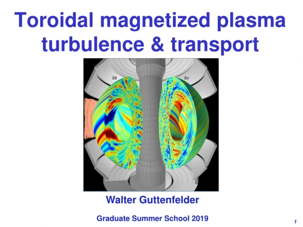
Toroidal magnetized plasma turbulence & transport Walter Guttenfelder Graduate Summer School 2019
Concepts of turbulence to remember • Turbulence is deterministic yet unpredictable (chaotic), appears random • Turbulence is not a property of the fluid / plasma, it’s a feature of the flow • We often treat & diagnose statistically, but also rely on first-principles direct numerical simulation (DNS) • Turbulence spans a wide range of spatial and temporal scales • Or in the case of hot, low-collisionality plasma, a wide range of scales in 6D phase-space (x,v) • Turbulence causes increased mixing, transport larger than collisional transport • Transport is the key application of why we care about turbulence • It’s cool! “Turbulence is the most important unsolved problem in classical physics” (~Feynman)
Coarse categorization of plasma turbulence • 3D MHD turbulence (Lecture #2) • Alfven waves in presence of guiding B field additional linear term • Derived in single-fluid MHD limit • Was done without consideration of strong variation in background B, n, T • 2D drift wave turbulence (today) • Driven by cross-field background thermal gradients (FM n, T) additional linear term + source of instability and microturbulence to relax gradients • Derived in two-fluid (two-species kinetic) limit • 2D toroidal drift wave turbulence (today) • Inhomogeneous B gives rise to B & curvature drifts and particle trapping additional dynamics for instability
Turbulent transport is an advective process • Transport a result of finite average 2nd order correlation between perturbed drift velocity (dv) and perturbed fluid moments (dn, dT, dv) • Particle flux, G = dvdn • Heat flux, Q = 3/2n0dvdT + 3/2T0dvdn • Momentum flux, P ~ dvdv (“Reynolds stress”) • Electrostatic turbulence often most relevant in tokamaks EB drift from potential perturbations: dvE=B(dj)/B2 ~ kq(dj)/B • Can also have magnetic contributions at high beta, dvB~v||(dBr/B) (magnetic “flutter” transport)
D-T fusion gain depends on the “triple product” nTtE Energy confinement time: Fusion plasma gain
Fusion gain depends on the “triple product” nTtE Energy confinement time: Fusion plasma gain Collisional transport, microturbulence, macroscopic instabilities, …
Charged particles experience Lorentz force in a magnetic field gyro-orbits • Magnetic force acts perpendicular to direction of particle Particles follow circular gyro-orbits B field into plane fc~ 107 / 1010 Hz (for deuteron / electron, B=5 T)
Magnetic field confines particles away from boundaries B 5 T T 10 keV gyroradius: Particles easily lost from ends bend into a torus Low collision frequency n~n/T3/2 lMFP~ km’s >> device size lMFP / ri ~ 106 c||/c ~ (lmfp/r)2~ 1012 (strong anisotropy) ri ~ 3 mm re~ 0.05 mm 1-2 meter device size <<
But toroidicity leads to vertical drifts from B & curvature tloss~ 5 msfrom vertical drifts (B~5 T, R~5 m, T~15 keV) + B - Key parameter in magnetized confinement
Even worse, charge separation leads to faster EB drifts out to the walls tloss~ msfrom EB drifts (due to charge separation from vertical drifts) z ɸ Btoroidal + + + Ion drift + E Electron drift - - - -
Solution: need a helical magnetic field for confined (closed) particle orbits a R R=major radius a=minor radius
Tokamaks NSTX • Toroidal, axisymmetric • Helical field lines confine plasma • Closed, nested flux surfaces
Tokamaks NSTX • Toroidal, axisymmetric • Helical field lines confine plasma • Closed, nested flux surfaces Heat loss
For what we’re going to discuss, general phenomenology also important for stellarators or any toroidal B field W7-X stellarator MST Reversed Field Pinch (RFP)
We use 1D transport equations for transport analysis • Take moments of plasma kinetic equation (Boltzmann Eq.) • Flux surface average, i.e. everything depends only on flux surface label (r) • Average over short space and time scales of turbulence (assume sufficient scale separation, e.gtturb << ttransport, Lturb << Lmachine) macroscopic transport equation for evolution of equilibrium (non-turbulent) plasma state (formally derived in limit of r*0) • To infer experimental transport, Qexp: • Measure profiles (Thomson Scattering, CHERS) • Measure / calculate sources (NBI, RF, fusion a’s) • Measure / calculate losses (Prad)
Inferred experimental transport larger than collisional (neoclassical) theory – extra “anomalous” contribution • Reporting transport as diffusivities – does not mean the transport processes are collisionally diffusive! TFTR Hawryluk, Phys. Plasmas (1998) Exp. Collisional theory
Spectroscopic imaging provides a 2D picture of turbulence in tokamaks: cm spatial scales, ms time scales, <1% amplitude • Beam Emission Spectroscopy (measures Doppler shifted Da from neutral beam heating to infer plasma density) DIII-D tokamak (General Atomics) Movies at: https://fusion.gat.com/global/BESMovies
Rough estimate of turbulent diffusivity indicates it’s a plausible explanation for confinement cturb ~ (Lcorr)2Dwdecorrelation Lcorr ~ few cm (~ ri) DwD ~ ~100 kHz (~vT/R) Pheat= Heat flux COLD HOT time-averaged temperature ~ cm’s instantaneous temperature core boundary ~1 m Turbulence confinement time estimate ~ 0.1 s Experimental confinement time ~ 0.1 s
40+ years of theory predicts turbulence in magnetized plasma should often be drift wave in nature General predicted drift wave characteristics: • Finite-frequency drifting waves, w(kq)~w*~kqV*~(kqr)vT/Ln • Driven by n, T (1/Ln = -1/nn) • Can propagate in ion or electron diamagnetic direction, depending on conditions/dominant gradients • Quasi-2D, elongated along the field lines (L||>>L, k|| << k ) • Particles can rapidly move along field lines to smooth out perturbations • Perpendicular sizes linked to local gyroradius, L~ri,e or kri,e~1 • Correlation times linked to acoustic velocity, tcor~cs/R • In a tokamak expected to be “ballooning”, i.e. stronger on outboard side • Due to “bad curvature”/”effective gravity” pointing outwards from symmetry axis • Often only measured at one location (e.g. outboard midplane) • Fluctuation strength loosely follows mixing length scaling (dn/n0~rs/Ln) • Transport has gyrobohmscaling, cGB=ri2vTi/R • But other factors important like threshold and stiffness: cturb ~ cGBF()[R/LT-R/LT,crit]
Ballooning nature observed in simulations (Hammett notes)
Transport is of order the Gyrobohm diffusivity • Although turbulence is advective, can estimate order of transport due to drift waves as a diffusive process L ~ rs tcorr-1 ~ cs/R • tE improves with field strength (B) and machine size (R) gyroBohm diffusivity Bohm diffusivity r* (have assumed R~a)
Tokamak turbulence has a threshold gradient for onset, transport tied to linear stability and nonlinear saturation • GyroBohm scaling important, but liner threshold and scaling also matters • We must discuss linear drift wave and micro-stability in tokamaks as part of the turbulent transport problem diffusion + turbulence Heat flux ~ heating power collisional diffusion Temperature gradient (-T)
Can identify key terms in “gyrofluid” equations responsible for drift wave dynamics • Start with toroidal GK equation in the df limit (df/FM << 1) • Take fluid moments • Apply clever closures that “best” reproduce linear toroidal gyrokinetics (Hammett, Perkins, Beer, Dorland, Waltz, …) Continuity and energy (M. Beer thesis, 1995): • Perturbed EB drift + background gradients (dvEn0, dvET0) are fundamental to drift wave dynamics
Simple classic electron drift wave in a magnetic slab (B=BZ) • Assume cool ions (vTi << w/k||), no temperature gradients, no toroidicity, no nonlinear term ion continuity Gradient scale length (Ln)
With some algebra we obtain a diamagnetic drift velocity & frequency Electron diamagnetic drift velocity & frequency (a fluid drift, not a particle drift) r* like parameter
Simplified ion continuity equation • Expect characteristic frequency ~ w*e ~ (kyrs)cs/Ln
Dynamics Must Satisfy Quasi-neutrality • Quasi-neutrality (Poisson equation, k2lD2<<1) requires • For characteristic drift wave frequency, parallel electron motion is very rapid -- from parallel electron momentum eq, assuming isothermal Te: • Electrons (approximately) maintain a Boltzmann distribution
Ion continuity + quasi-neutrality + Boltzmann electron = electron drift wave (linear, slab, cold ions) • Density and potential wave perturbations propagating perpendicular to BZ and n0 • dvEn0 gives dn 90° out-of-phase with initial dnperturbation • Simple linear dispersion relation (will change with polarization drift / finite Larmor radius effects, toroidicity, other graidents) • No mechanism to drive instability (collisions, temperature gradient, toroidicity / trapped particles, …)
Gyrokinetic simulations find that nonlinear transport follows many of the underlying linear instability trendsVery valuable to understand linear instabilities Example: Linear stability analysis of toroidal Ion Temperature Gradient (ITG) micro-instability (expected to dominate in ITER)
Toroidicity Leads To Inhomogeneity in |B|, gives B and curvature (k) drifts • What happens when there are small perturbations in T||, T? Linear stability analysis… B, curvature (k) Z Z R R
Temperature perturbation (dT) leads to compression (vdi), density perturbation – 90 out-of-phase with dT • Fourier decompose perturbations in space (kqri1) • Assume small T perturbation B, curvature T+ T- T+ T- T+ T- n- n+ n- n+ n- B T n T
Dynamics Must Satisfy Quasi-neutrality • Quasi-neutrality (Poisson equation, k2lD2<<1) requires • For characteristic drift wave frequency, parallel electron motion is very rapid (from parallel electron momentum eq, assuming isothermal Te:) • Electrons (approximately) maintain a Boltzmann distribution
Perturbed Potential Creates EB Advection • Advection occurs in the radial direction B, curvature ~Boltzmann e’s T+ T- T+ T- T+ T- - + - + - n- n+ n- n+ n- E E E E B T n T
Background Temperature Gradient Reinforces Perturbation Instability T T+ T- T+ T- T+ T- This simple cartoon gives a purely growing “interchange” like mode (coarse derivation in backup slides). The complete derivation (all drifts, gradients) will give a real frequency.
Analogy for turbulence in tokamaks – Rayleigh-Taylor instability • Higher density on top of lower density, with gravity acting downwards gravity density/pressure
Inertial force in toroidal field acts like an effective gravity centrifugal force effective gravity gravity pressure pressure Unstable in the outer region GYRO code https://fusion.gat.com/theory/Gyro
Same Dynamics Occur On Inboard Side But Now Temperature Gradient Is Stabilizing • Advection with T counteracts perturbations on inboard side – “good” curvature region “good” curvature “bad” curvature T T B T+ T- T+ T- T+ T- T+ T- T+ T- T+ T- T n T T
Similar to comparing stable / unstable (inverted) pendulum (Hammett notes)
Fast Parallel Motion Along Helical Field Line Connects Good & Bad Curvature Regions • Approximate growth rate on outboard side effective gravity: geff = vth2/R gradient scale length: 1/LT = -1/TT • Parallel transit time along helical field line with “safety factor” q • Expect instability if ginstability > gparallel , or
Helical B field carries plasma from “bad curvature” region to “good curvature” region Similar to how honey dipper prevents honey from dripping
Threshold-like behavior analogous to Rayleigh-Benard instability Analogous to convective transport when heating a fluid from below … boiling water (before the boiling) Heat flux ~ heating power diffusion + turbulence collisional diffusion Rayleigh, Benard, early 1900’s Temperature gradient (Thot - Tcold)
Threshold-like behavior observed experimentally • Experimentally inferred threshold varies with equilibrium, plasma rotation, ... • Stiffness (~dQ/dT above threshold) also varies • c = -Q/nT highly nonlinear (also use perturbative experiments to probe stiffness) JET Mantica, PRL (2011)
With physical understanding, can try to manipulate/optimize microstability • E.g., magnetic shear influences stability by twisting radially-elongated instability to better align (or misalign) with bad curvature drive Antoneson
Reverse magnetic shear can lead to internal transport barriers (ITBs) • ITBs established on numerous devices • Used to achieve “equivalent” QDT,eq~1.25 in JT-60U (in D-D plasma) • ci~ci,NC in ITB region (complete suppression of ion scale turbulence) JT-60U Ishida, NF (1999)
Critical gradient for ITG determined from many linear gyrokinetic simulations (guided by theory) • R/LT = -R/TT is the normalized temperature gradient • Natural way to normalize gradients for toroidal drift waves, i.e. ratio of diamagnetic-to-toroidal drift frequencies: w*T = ky(B×p) / nqB2 (kqri)vT/LT wD = ky(B×mv2B/2B) / qB2 (kqri)vT/R Jenko (2001) Hahm (1989) Romanelli (1989) w*T/wD = R/LT
How does magnetized turbulence saturate?What sets spatial scales (drive vs. dissipation)?


