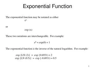
The Natural Exponential Function
The Natural Exponential Function. Natural Exponential Function. Any positive number can be used as the base for an exponential function. However, some are used more frequently than others.

The Natural Exponential Function
E N D
Presentation Transcript
Natural Exponential Function • Any positive number can be used as the base for an exponential function. • However, some are used more frequently than others. • We will see in the remaining sections of the chapter that the bases 2 and 10 are convenient for certain applications. • However, the most important is the number denoted by the letter e.
Number e • The number e is defined as the value that (1 + 1/n)n approaches as n becomes large. • In calculus, this idea is made more precise through the concept of a limit.
Number e • The table shows the values of the expression (1 + 1/n)nfor increasingly large values of n. • It appears that, correct to five decimal places, e ≈ 2.71828
Number e • The approximate value to 20 decimal places is: e≈ 2.71828182845904523536 • It can be shown that e is an irrational number. • So, we cannot write its exact value in decimal form.
Number e • Why use such a strange base for an exponential function? • It may seem at first that a base such as 10 is easier to work with. • However, we will see that, in certain applications, itis the best possible base.
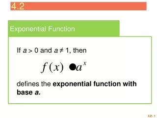
Natural Exponential Function—Definition • The natural exponential functionis the exponential function f(x) = exwith base e. • It is often referred to as theexponential function.
Natural Exponential Function • Since 2 < e < 3, the graph of the natural exponential function lies between the graphs of y = 2xand y = 3x.
Natural Exponential Function • Scientific calculators have a special key for the function f(x) = ex. • We use this key in the next example.
E.g. 6—Evaluating the Exponential Function • Evaluate each expression correct to five decimal places. • (a) e3 • (b) 2e–0.53 • (c) e4.8
E.g. 6—Evaluating the Exponential Function • We use the ex key on a calculator to evaluate the exponential function. • e3≈ 20.08554 • 2e–0.53≈ 1.17721 • e4.8≈ 121.51042
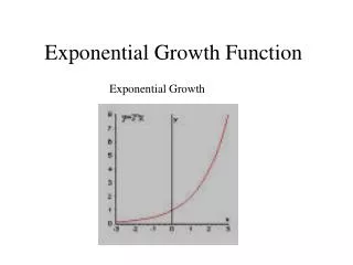
E.g. 7—Transformations of the Exponential Function • Sketch the graph of each function. • f(x) = e–x • g(x) = 3e0.5x
Example (a) E.g. 7—Transformations • We start with the graph of y =exand reflect in the y-axis to obtain the graph of y =e–x.
Example (b) E.g. 7—Transformations • We calculate several values, plot the resulting points, and then connect the points with a smooth curve.
E.g. 8—An Exponential Model for the Spread of a Virus • An infectious disease begins to spread in a small city of population 10,000. • After t days, the number of persons who have succumbed to the virus is modeled by:
E.g. 8—An Exponential Model for the Spread of a Virus • How many infected people are there initially (at time t = 0)? • Find the number of infected people after one day, two days, and five days. • Graph the function v and describe its behavior.
Example (a) E.g. 8—Spread of Virus • We conclude that 8 people initially have the disease.
Example (b) E.g. 8—Spread of Virus • Using a calculator, we evaluate v(1), v(2), and v(5). • Then, we round off to obtain these values.
Example (c) E.g. 8—Spread of Virus • From the graph, we see that the number of infected people: • First, rises slowly. • Then, rises quickly between day 3 and day 8. • Then, levels off when about 2000 people are infected.
Logistic Curve • This graph is called a logistic curveor a logistic growth model. • Curves like it occur frequently in the study of population growth.
Compound Interest • Exponential functions occur in calculating compound interest. • Suppose an amount of money P, called the principal, is invested at an interest rate i per time period. • Then, after one time period, the interest is Pi, and the amount A of money is:A = P + Pi + P(1 + i)
Compound Interest • If the interest is reinvested, the new principal is P(1 + i), and the amount after another time period is: A = P(1 + i)(1 + i) = P(1 + i)2 • Similarly, after a third time period, the amount is: A = P(1 + i)3
Compound Interest • In general, after k periods, the amount is: A = P(1 + i)k • Notice that this is an exponential function with base 1 + i.
Compound Interest • Now, suppose the annual interest rate is r and interest is compounded n times per year. • Then, in each time period, the interest rate is i =r/n, and there are nt time periods in t years. • This leads to the following formula for the amount after t years.
Compound Interest • Compound interestis calculated by the formulawhere: • A(t) = amount after t years • P = principal • t = number of years • n = number of times interest is compounded per year • r = interest rate per year
E.g. 9—Calculating Compound Interest • A sum of $1000 is invested at an interest rate of 12% per year. • Find the amounts in the account after 3 years if interest is compounded: • Annually • Semiannually • Quarterly • Monthly • Daily
E.g. 9—Calculating Compound Interest • We use the compound interest formula with: P = $1000, r = 0.12, t = 3
Compound Interest • We see from Example 9 that the interest paid increases as the number of compounding periods n increases. • Let’s see what happens as n increases indefinitely.
Compound Interest • If we let m = n/r, then
Compound Interest • Recall that, as m becomes large, the quantity (1 + 1/m)m approaches the number e. • Thus, the amount approaches A =Pert. • This expression gives the amount when the interest is compounded at “every instant.”
Continuously Compounded Interest • Continuously compounded interestis calculated by A(t) = Pert • where: • A(t) =amount after t years • P = principal • r = interest rate per year • t = number of years
E.g. 10—Continuously Compounded Interest • Find the amount after 3 years if $1000 is invested at an interest rate of 12% per year, compounded continuously.
E.g. 10—Continuously Compounded Interest • We use the formula for continuously compounded interest with: P = $1000, r = 0.12, t = 3 • Thus, A(3) = 1000e(0.12)3 = 1000e0.36 = $1433.33 • Compare this amount with the amounts in Example 9.