Download

1 / 23
250 likes | 407 Views
ELEC 303 – Random Signals. Lecture 20 – Random processes Dr. Farinaz Koushanfar ECE Dept., Rice University Nov 11, 2010. Lecture outline. Basic concepts Random processes and linear systems Power spectral density of stationary processes Power spectra in LTI systems

E N D
ELEC 303 – Random Signals Lecture 20 – Random processes Dr. Farinaz Koushanfar ECE Dept., Rice University Nov 11, 2010
Lecture outline • Basic concepts • Random processes and linear systems • Power spectral density of stationary processes • Power spectra in LTI systems • Power spectral density of a sum process • Gaussian processes
RP and linear systems • When a RP passes a linear time-invariant system the output is also a RP • Assuming a stationary process X(t) is input, the linear time-invariant system with the impulse response h(t), output process Y(t) • Under what condition the output process would be stationary? • Under what conditions will the input/output jointly stationary? • Find the output mean, autocorrelation, and crosscorrelation h(t) X(t) Y(t)
Linear time invariant systems • If a stationary RP with mean mX and autocorrelation function RX() • Linear time invariant (LTI) system with response h(t) • Then, the input and output process X(t) and Y(t) will be jointly stationary with h(t) X(t) Y(t)
The response mean • Using the convolution integral to relate the output Y(t) to the input X(t), Y(t)=X()h(t-)d This proves that mY is independent of t h(t) X(t) Y(t)
Cross correlation • The cross correlation function between output and the input is This shows that RXY(t1,t2) depends only on =t1-t2
Output autocorrelation • The autocorrelation function of the output is This shows that RY and RXY depend only on =t1-t2, Output process is stationary, and input/output are jointly stationary
Power spectral density of a stationary process • If the signals in the RP are slowly varying, then the RP would mainly contain the low frequencies in its power concentration • If the signal changes very fast, most of the power will be concentrated at high frequency • The power spectral density of a RP X(t) is denoted by SX(f) showing the strength of the power in RP as a function of frequency • The unit for SX(f) is Watts/Hz
Wiener-Khinchin theorem • For a stationary RP X(t), the power spectral density is the Fourier transform of the autocorrelation function, i.e.,
Example 2 • Randomly choose a phase ~ U[0,2] • Generate a sinusoid with fixed amplitude (A) and fixed freq (f0) but a random phase • The RP is X(t)= A cos(2f0t + ) • From the previous lecture, we know
Example 3 • X(t)=X • Random variable X~U[-1,1] • In this case • Thus, • For each realization of the RP, we have a different power spectrum
Power spectral density • The power content of a RP is the sum of the powers at all frequencies in that RP • To find the total power, need to integrate the power spectral density across all frequencies • Since SX(f) is the Fourier transform of RX(), then RX() will be the inverse Fourier transform of SX(f), Thus • Substituting =0, we get
Example 4 • Find the power in the process of example 2
Translation to frequency domain • For the LTI system and stationary input, find the translation of the relationships between the input/output in frequency domain • Compute the Fourier transform of both sides to obtain • Which says the mean of a RP is its DC value. Also, phase is irrelevant for power. Only the magnitude affects the power spectrum, i.e., power dependent on amplitude, not phase
Example 5 • If a RP passes through a differentiator • H(f)=j2f • Then, mY=mX H(0) = 0 • Also, SY(f) = 42 f2 SX(f)
Cross correlation in frequency domain • Let us define the cross spectral density SXY(f) • Since RYX() = RXY(-), we have • Although SX(f) and SY(f) are real nonnegative functions, SXY(f) and SYX(f) can generally be complex functions
Example 6 • Randomly choose a phase ~ U[0,2] • Generate a sinusoid with fixed amplitude (A) and fixed freq (f0) but a random phase • The RP is X(t)= A cos(2f0t + ) • The X(t) goes thru a differentiator H(f)=j2f
Example 7 • X(t)=X • Random variable X~U[-1,1] • If this goes through differentiation, then SY(f) = 42 f2 ((f)/3) = 0 SXY(f) = -j2f ((f)/3) = 0
Power spectral density of a sum process • Z(t) = X(t)+Y(t) • X(t) and Y(t) are jointly stationary RPs • Z(t) is a stationary process with RZ() = RX() + RY() + RXY() + RYX() • Taking the Fourier transform from both sides: SZ(f) = SX(F) + SY(f) + 2 Re[SXY(f)] • The power spectral density of the sum process is the sum of the power spectral of the individual processes plus a term, that depends on the cross correlation • If X(t) and Y(t) are uncorrelated, then RXY()=mXmY • If at least one of the processes is zero mean, RXY()=0, and we get: SZ(f) = SX(F) + SY(f)
Example 8 • X(t)=X • Random variable X~U[-1,1] • Z(t) = X(t) + d/dt X(t), then • SXY(f) = jA2f0 /2 [(f+f0) - (f-f0)] • Thus, • Re[SXY(f)] = 0 • SZ(f)= SX(f)+SY(f) = A2(1/4+2f02)[(f+f0)+(f-f0)]
Gaussian processes • Widely used in communication • Because thermal noise in electronics is produced by the random movement of electrons closely modeled by a Gaussian RP • In a Gaussian RP, if we look at different instances of time, the resulting RVs will be jointly Gaussian: Definition 1: A random process X(t) is a Gaussian process if for all n and all (t1,t2,…,tn), the RVs {X(ti)}, i=1,…,n have a jointly Gaussian density function.
Gaussian processes (Cont’d) • It is obvious that if X(t) and Y(t) are jointly Gaussian, then each of them is individually Gaussian • The reverse is not always true • The Gaussian processes have important and unique properties Definition 2: The random processes X(t) and Y(t) are jointly Gaussian if for all n and all (t1,t2,…,tn), and (1,2,…,m)the random vector {X(ti)}, i=1,…,n, {Y(j}, j=1,…,m have an n+m dimensional jointly Gaussian density function.
Important properties of Gaussian processes • Property 1: If the Gaussian process X(t) is passed through an LTI system, then the output process Y(t) will also be a Gaussian process. Y(t) and X(t) will be jointly Gaussian processes • Property 2: For jointly Gaussian processes, uncorrelatedness and independence are equivalent