Download
1 / 54
540 likes | 824 Views
Modeling Larval Dispersal on the Southeast U.S. Continental Shelf: Implications for Marine Protected Area design. Karen Pehrson Edwards Research Seminar 9 February 2005. Outline. Background: MPAs & Larval Dispersal Study Area: SEUSCS and Grays Reef National Marine Sanctuary (GRNMS)

E N D
Modeling Larval Dispersal on the Southeast U.S. Continental Shelf: Implications for Marine Protected Area design Karen Pehrson Edwards Research Seminar 9 February 2005
Outline Background: MPAs & Larval Dispersal Study Area: SEUSCS and Grays Reef National Marine Sanctuary (GRNMS) Models & Results Next Steps
State of Fisheries • FAO World Fisheries Report: • 1998 • 69% of the world’s marine fish stocks are “fully exploited, overexploited or depleted” • 2002 • 75% of the world’s marine fish stocks are “fully exploited, overexploited or depleted” • Snapper-Grouper Management Unit of the South Atlantic Fishery Management Council • 17.8% overfished/overfishing • 13.7% not overfished/no overfishing • 68.5% status UNKNOWN
Marine Managed Areas • Federal Regulation: • Fish and Wildlife Coordination Act (1934) • National Wildlife Refuge System Administration Act (1966) • Coastal Zone Management Act (1972, Amended in 1996) • Endangered Species Act (1973) • Magnuson-Stevens Fishery Conservation & Management Act (1976, amended 1996) • National Marine Sanctuary Act (1976, last updated in 1992) • Management responsibilities exist in several agencies within both the Department of Commerce and the Department of the Interior. • There are more than 100 state, territorial, and commonwealth agencies with area-based management authority. www.mpa.gov
The nation’s collection of marine managed areas is complex and confusing! Generated from the Marine Managed Areas Inventory Atlas. [source: www.MPA.gov]
Marine Protected Areas • Executive Order 13158 (2000) created a framework for a national system of MPAs • Provides:management, protection and conservation for existing MPAs and ability to create new ones. • Does not:designate new sites, create new authorities or change existing ones, focus solely on “no-take” reserves or set specific targets for habitat protection. • U.S. Commission on Ocean Policy (2004) • Guiding Principles: • Sustainability • Recommendations for Sustainable Fisheries: • Re-emphasizing the role of science in the management process, • Adopting an ecosystem-based management approach.
Marine Protected Areas MPA’s in Theory Increased proportion of larger/older individuals Increased abundance Recolonization of habitats Population pressures -> emigration of adults to fished areas outside MPA Increased supply of eggs and larvae Increased number of predators Increased competition for food/habitat Export of eggs and larvae to surrounding areas Density dependence Increased recruitment inside MPA Increased mortality of recruits Increased recruitment outside MPA Adapted from the FAO Fisheries Technical Report 448
Larval Dispersal Paradigm - Marine populations are open Larval dispersal connects local populations over large distances • Supporting Evidence • Genetic similarity of widely spaced populations • Simple passive drift models • Problems with this Evidence • Genetic homogeneity only requires exchange of a few individuals per generation • Larvae are not passive, flow is not simple From Robert Cowen presentation November 2002
Larval Dispersal Single, patchy Separate population populations HighLow (open)Population Connectivity (closed) Connectivity is the measure of the rates of exchange of individuals among sub-populations Modified from Harrison and Taylor (1997) From Robert Cowen presentation November 2002
Dispersal Scenarios Dispersal Kernel: probability of ending up at x given a starting point of y Number of recruits Active Retention Simple Diffusion Passive, Mean Flow- Diffusion y Distance downstream(x)
Dispersal Scenarios Broadly Dispersed (Open) Local Retention (Closed) Population Connectivity No. of Recruits from Source y Distance from Source (x) From Robert Cowen presentation November 2002
1 2 3 4 1 2 3 4 Number of local sources Multiple Single Larval Pool 1 2 3 4 1 2 3 4 Short Long Distance of propagule dispersal Larval Dispersal and MPA design A C B D Allison et al, 1998
1 2 3 4 Reserve 3 4 1 2 Reserve Allison et al, 1998 Larval Dispersal and MPA design C
Sea Scallop Transport andClosed Area Analyses From John Quinlan ECOHAB/GLOBEC Portland, ME -June 17-18, 2000
Closed Areas I and II act in such a way as to be both self seeding and source populations for one another… And settlement areas seem to match observation… From John Quinlan ECOHAB/GLOBEC Portland, ME -June 17-18, 2002
Research Questions • Determine the source regions providing recruitment to GRNMS and the supply regions receiving recruitment from GRNMS. • What are the implications to designing a network of Marine Protected Areas (MPAs) on the Southeast U.S. Continental Shelf?
Southeast U.S. Continental Shelf • Cape Hatteras, NC south to Cape Canaveral, FL • From 40 to 140 km wide • 30% rocky-reefs which support more than 70% of the offshore fisheries Provided by Harvey Walsh, NOAA Beaufort
Southeast U.S. Continental Shelf Inner Shelf (<15-20m): • River runoff • Atmospheric fluxes and tides Mid- Shelf (20-40m): • Winds • Tides and Gulf Stream Outer- Shelf (>40m): • Gulf Stream http://www.skio.peachnet.edu/ Lee et al. 1991
Grays Reef National Marine Sanctuary Located 32 km off Sapelo Island, GA Encompasses 58 km2 of rocky-reef habitat. Designated a National Marine Sanctuary in 1981 http://sablam.unc.edu/maps.html
Research Approach • Couple physical and biological modeling to define the dispersal kernels of fish larvae on the SEUSCS • 1st step: Evaluate circulation model using observed drifter tracks: • 26 April 2000 • 21 June 2000 • 3 October 2000 • 30 January 2001 • 22 March 2001
3-D Circulation Model • QUODDY • Forced with winds (NCEP EDAS) and tides • Provides velocity fields for particle tracking • Compare: • Water level • Currents Lynch et al., 1996
Model Results – Water Level April 2000: best drifter fit rms = 0.08m rms = 0.067m June 2000: worst drifter fit rms = 0.082m rms = 0.077m
Model Results – Velocity April 2000: best drifter fit rms = 0.069m/s rms = 0.052m/s June 2000: worst drifter fit rms = 0.14m/s rms = 0.045m/s
Particle Tracking Model • Time-stepping version of the Lagrangian tracking algorithm (Blanton,1993) with modifications (Edwards et al., in prep) • QUODDY 3D velocity fields as input • Numerical drifters started at the time and location of the first satellite record from the observed drifters
Particle Tracking: Oct 2000 • Sources of Error • Winds • River discharge • Gulf Stream • Baroclinic flow • Drifter Behavior • What can we account for? • Winds • Drifter Behavior
Particle Tracking Model • Modification for differences in the EDAS and observed wind fields Generally, the EDAS model product underestimates the observed winds, hence, the ocean model generally underpredicts observed currents.
Wind Comparison SABSOON R2 m2/s2/Hz M2/s2/Hz Oct 2000 Blanton, 2003
Modification for differences in EDAS and observed wind stress http://www.personal.psu.edu/users/m/j/mjr300/481.html
Particle Tracking Model • Modification due to drifter slippage 10m Pictures provided by Jon Hare.
Modification for Drifter Slippage • Wind drag on the float, • Current drag on the submerged part of the float, • Current drag on the tether and the drogue, • And nonlinear wave action (Geyer, 1989) 10m Picture provided by Jon Hare.
ParticleTracking Model • The total velocity acting on the numerical drifters is then given by: Udrifter=UQUODDY+Uekman+Uslip
Model Comparison Separation = distance between numerical and observed drifters
Model Comparison Separation = distance between numerical and observed drifters
Drifter separation Separation Rate = change in separation distance over time
Model Summary • 3D Circulation Model (QUODDY) captures the dynamics of the shelf. • Particle tracking model with modifications for drifter slip and wind stress differences provides a good fit for observed drifters. • Separation rate ≤ 2km/day
Next Steps • Move from modeling drifters to larvae • Remove drifter behavior from particle tracking model • Begin to define the dispersal kernels of larvae released on the SEUSCS • Gag grouper: Winter-Spring • Black sea bass: Spring
Passive, Mean Flow- Diffusion Next Steps: Define Dispersal Kernels
What affects the shape of the dispersal kernel? • Physical factors: • Passive advection and diffusion • Intermittent/episodic events • Interannual variability • Long-term modulations (ENSO,NAO) • Compare several years of model dispersal and climatology for a given dispersal period (March-May).
What affects the shape of the dispersal kernel? • Biological Factors: • Larval Behavior • Along-trajectory mortality: feeding, predation, physical environment • Include larval behavior in the dispersal scenarios.
Larval Behavior Low High Behavioral Capacity From Robert Cowen presentation November 2002
Larval Behavior Model Explore implications of various behaviors • Ontogenetic shifts… • Diel vertical migration… Hare et al. (1999)
Larval Behavior Model Hare et al. (1999)
Dispersal from Mutton Snapper Spawning Aggregations From Robert Cowen presentation November 2002
Next Steps:Incorporate larval selection of suitable bottom habitat into the dispersal kernels. Provided by Harvey Walsh, NOAA Beaufort