Download
1 / 6
70 likes | 214 Views
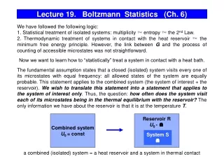
Delve into the statistical treatment of isolated systems, the link between entropy and free energy, and the principle of thermal equilibrium. Explore how systems interact with heat reservoirs with equal frequency and the implications of the ergodic hypothesis. Learn about the macroscopic and microscopic aspects of system behavior in thermodynamic equilibrium.

E N D
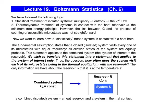
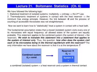
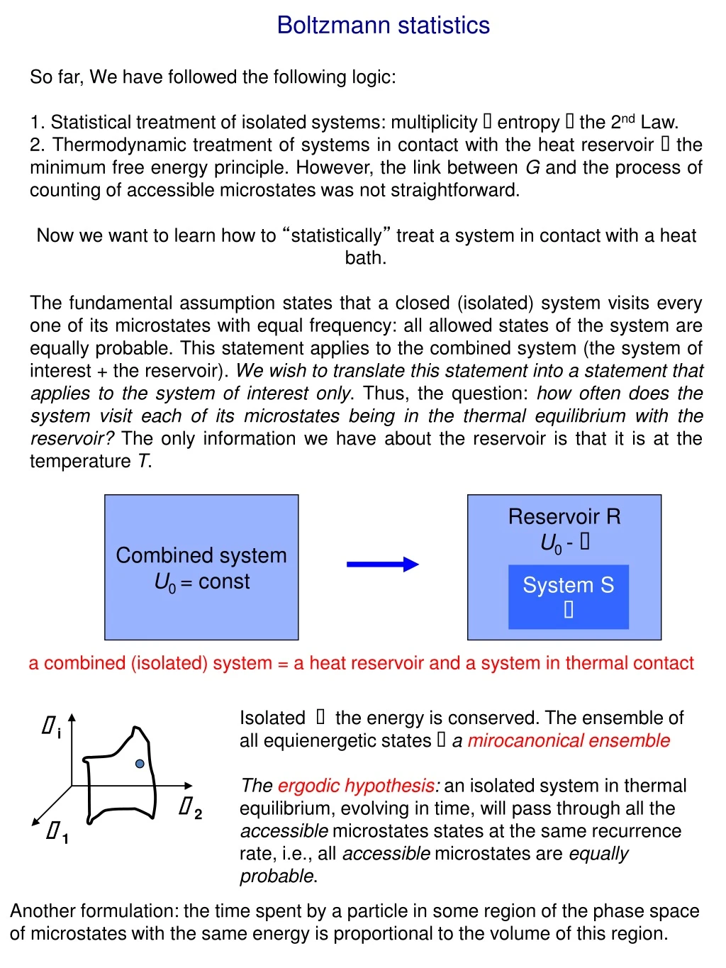
Boltzmann statistics So far, We have followed the following logic: 1. Statistical treatment of isolated systems: multiplicity entropy the 2nd Law. 2. Thermodynamic treatment of systems in contact with the heat reservoir the minimum free energy principle. However, the link between G and the process of counting of accessible microstates was not straightforward. Now we want to learn how to “statistically” treat a system in contact with a heat bath. The fundamental assumption states that a closed (isolated) system visits every one of its microstates with equal frequency: all allowed states of the system are equally probable. This statement applies to the combined system (the system of interest + the reservoir). We wish to translate this statement into a statement that applies to the system of interest only. Thus, the question: how often does the system visit each of its microstates being in the thermal equilibrium with the reservoir? The only information we have about the reservoir is that it is at the temperature T. Combined system U0 = const Reservoir R U0 - System S a combined (isolated) system = a heat reservoir and a system in thermal contact Isolated the energy is conserved. The ensemble of all equienergetic states a mirocanonical ensemble The ergodic hypothesis:an isolated system in thermal equilibrium, evolving in time, will pass through all the accessible microstates states at the same recurrence rate, i.e., all accessible microstates are equally probable. i 2 1 Another formulation: the time spent by a particle in some region of the phase space of microstates with the same energy is proportional to the volume of this region.
The average over long times will equal the average over the ensemble of all equienergetic microstates: if we take a snapshot of a system with N microstates, we will find the system in any of these microstates with the same probability. Probability of a particular microstate of a microcanonical ensemble = 1 / (# of all accessible microstates) The probability of a certain macrostate is determined by how many microstates correspond to this macrostate – the multiplicity of a given macrostate macrostate Probability of a particular macrostate = ( of a particular macrostate) / (# of all accessible microstates) Note that the assumption that a system is isolated is important. If a system is coupled to a heat reservoir and is able to exchange energy, in order to replace the system’s trajectory by an ensemble, we must determine the relative occurrence of states with different energies. In macroscopic systems, the timescales over which a system can truly explore the entirety of its own phase space can be sufficiently large that the thermodynamic equilibrium state exhibits some form of ergodicity breaking. A common example is that of spontaneous magnetisation in ferromagnetic systems, whereby below the Curie temperature the system preferentially adopts a non-zero magnetisation even though the ergodic hypothesis would imply that no net magnetisation should exist by virtue of the system exploring all states whose time-averaged magnetisation should be zero. The fact that macroscopic systems often violate the literal form of the ergodic hypothesis is an example of spontaneous symmetry breaking.
SR S(U0) S(U0- 1) S(U0- 2) UR U0 U0- 1 U0- 2 The system: any small macroscopic or microscopic object. If the coupling between the system and the reservoir is weak, we can assume that the spectrum of energy levels of a weakly-interacting system is the same as that for an isolated system. We ask the following question: under conditions of equilibrium between the system and reservoir, what is the probability P(k) of finding the system S in a particular quantum state k of energy k? We assume weak coupling between R and S so that their energies are additive. The energy conservation in the isolated system “system + reservoir”: U0 = UR+ US = const According to the fundamental assumption of thermodynamics, all the states of the combined (isolated) system “R+S” are equally probable. By specifying the microstate of the system k, we have reduced Sto 1 and SS to 0. Thus, the probability of occurrence of a situation where the system is in state k is proportional to the number of states accessible to the reservoirR . The total multiplicity: The ratio of the probability that the systemis in quantum state 1 at energy 1to the probability that the system is in quantum state 2 at energy 2is: Let’s now use the fact that S is much smaller than R (US=k ≪UR). Also, we will consider the case of fixed volume and number of particles (the latter limitation will be removed later, when we will allow the system to exchange particles with the heat bath).
T is the characteristic of the heat reservoir The quantity exp(- k/kBT) is called the Boltzmann factor. The Boltzmann factor is not a probability by itself, because it is not normalized. The normalization factor is one divided by the partition function, the sum of the Boltzmann factors for all states of the system. This gives the Boltzmann distribution. To quote Planck, "The logarithmic connection between entropy and probability was first stated by L. Boltzmann in his kinetic theory of gases". Ludwig Eduard Boltzmann (1844 – 1906) Wahrscheinlichkeit, the frequency of occurrence of a macrostate
This result shows that we do not have to know anything about the reservoir except that it maintains a constant temperature T. The corresponding probability distribution is known as the canonical distribution. An ensemble of identical systems all of which are in contact with the same heat reservoir and distributed over states in accordance with the Boltzmann distribution is called a canonical ensemble. The fundamental assumption for an isolated system has been transformed into the following statement for the system of interest which is in thermal equilibrium with the thermal reservoir: the system visits each microstate with a frequency proportional to the Boltzmann factor. Apparently, this is what the system actually does, but from the macroscopic point of view of thermodynamics, it appears as if the system is trying to minimize its free energy. Or conversely, this is what the system has to do in order to minimize its free energy. The lowest energy level 0 available to a system (e.g., a molecule) is referred to as the “ground state”. If we measure all energies relative to 0 and n0 is the number of molecules in this state, than the number molecules with energy > 0 reservoir T Problem 6.14. Use Boltzmann factors to derive the exponential formula for the density of an isothermal atmosphere. The system is a single air molecule, with two states: 1 at the sea level (z = 0), 2 – at a height z. The energies of these two states differ only by the potential energy mgz (the temperature T does not vary with z):
The Partition Function For the absolute values of probability (rather than the ratio of probabilities), we need an explicit formula for the normalizing factor 1/Z: - we will often use this notation The quantity Z, the partition function, can be found from the normalization condition - the total probability to find the system in all allowed quantum states is 1: Zustandssumme (sum over states) in German The partition function Z is called “function” because it depends on T, the spectrum (thus, V),etc. Example: a single particle, continuous spectrum. (kT1)-1 At T = 0, the system is in its ground state (=0) with the probability =1. T1 T2 (kT2)-1 0