Download

1 / 32
330 likes | 706 Views
Deep Boltzmann Machines. Salakhutdinov , Hinton International Conference on Artificial Intelligence and Statistics (AISTATS) 2009. 1 Introduction. The original learning algorithm for Boltzmann machines (Hinton and Sejnowski , 1983) was too slow to be practical.

E N D
Deep Boltzmann Machines Salakhutdinov, Hinton International Conference on Artificial Intelligence and Statistics (AISTATS) 2009
1 Introduction • The original learning algorithm for Boltzmann machines (Hinton and Sejnowski, 1983) was too slow to be practical. • Learning can be made much more efficient in a restricted Boltzmann machine (RBM) (2002). • Multiple hidden layers can be learned by treating the hidden activities of one RBM as the data for training a higher-level RBM (Hinton et al., 2006). • If multiple layers are learned in this greedy, layer-by-layer way, the resulting composite model is not a multilayer Boltzmann machine (Hinton et al., 2006). It is a hybrid generative model called a “deep belief net” that has undirected connections between its top two layers and downward directed connections between all its lower layers. • In this paper we present a much more efficient learning procedure for fully general Boltzmann machines. 1
2 Boltzmann Machines (BM’s) • A Boltzmann machine is a network of symmetrically coupled stochastic binary units. • It contains a set of visible units v{0, 1}D, and a set of hidden units h{0, 1}P 1
The energy of the state {v, h} • W, L, J: symmetric • Lii=0 , Jii=0, for all i. • The probability that the model assigns to a visible vector v 1
The conditional distributions over hidden and visible units • The parameter updates (1983), can be obtained from (2) by gradient ascent in the log-likelihood 1
Exact maximum likelihood learning in this model is intractable because exact computation of both the data dependent expectations and the model’s expectations takes a time that is exponential in the number of hidden units. • Hinton et al (1983) proposed an algorithm that uses Gibbs sampling to approximate both expectations. For each iteration of learning, a separate Markov chain is run for every training data vector to approximate EPdata [·], and an additional chain is run to approximate EPmodel [·]. • the time required to approach the stationary distribution, especially when estimating the model’s expectations. • the Gibbs chain may need to explore a highly multimodal energy landscape. • Setting both J=0 and L=0 recovers the restricted Boltzmann machine (RBM) model (Smolensky, 1986) (see Fig. 1, right panel). • In contrast to general BM’s, inference in RBM’s is exact. • Although exact maximum likelihood learning in RBM’s is still intractable, learning can be carried out efficiently using Contrastive Divergence (CD) (Hinton, 2002). • Many persistent chains can be run in parallel and we will refer to the current state in each of these chains as a “fantasy” particle. 1
For Contrastive Divergence to perform well, it is important to obtain exact samples from the conditional distribution p(h|v;), which is intractable when learning full Boltzmann machines. 2.1 Using Persistent Markov Chains to Estimate the Model’s Expectations • Instead of using CD learning, it is possible to make use of a stochastic approximation procedure (SAP) to approximate the model’s expectations (Tieleman, 2008). • SAP belongs to the class of well-studied stochastic approximation algorithms of the Robbins–Monro type. • Let t and Xt be the current parameters and the state. Then t and Xt are updated sequentially as follows: • Given Xt, a new state Xt+1 is sampled from a transition operator Tt(Xt+1;Xt) that leaves pt invariant. • A new parameter t+1 is then obtained by replacing the intractable model’s expectation by the expectation with respect to Xt+1. • One necessary condition requires the learning rate to decrease with time, i.e. 1
The intuition behind why this procedure works • as the learning rate becomes sufficiently small compared with the mixing rate of the Markov chain, this “persistent” chain will always stay very close to the stationary distribution even if it is only run for a few MCMC updates per parameter update. • Samples from the persistent chain will be highly correlated for successive parameter updates, but again, if the learning rate is sufficiently small the chain will mix before the parameters have changed enough to significantly alter the value of the estimator. • Many persistent chains can be run in parallel. 1
2.2 A Variational Approach to Estimating the Data- Dependent Expectations • In variational learning (Hinton and Zemel, 1994), the true posterior distribution over latent variables p(h|v; ) for each training vector v, is replaced by an approximate posterior q(h|v; μ) and the parameters are updated to follow the gradient of a lower bound on the log-likelihood: • in addition to trying to maximize the log-likelihood of the training data, it tries to find parameters that minimize the Kullback–Leibler divergences between the approximating and true posteriors. 1
we choose a fully factorized distribution in order to approximate the true posterior: • The learning proceeds by maximizing this lower bound with respect to the variational parameters μ for fixed , which results in mean-field fixed-point equations: 1
This is followed by applying SAP to update the model parameters (Salakhutdinov, 2008). • Variational approximations cannot be used for approximating the expectations with respect to the model distribution in the Boltzmann machine learning rule because the minus sign (see Eq. 6) would cause variational learning to change the parameters so as to maximize the divergence between the approximating and true distributions. • If, however, a persistent chain is used to estimate the model’s expectations, variational learning can be applied for estimating the data-dependent expectations. • Advantage of this method • First, the convergence is usually very fast. • Second, for applications such as the interpretation of images or speech, we expect the posterior over hidden states given the data to have a single mode, so simple and fast variational approximations such as mean-field should be adequate. • sacrificing some log-likelihood in order to make the true posterior unimodal could be advantageous for a system that must use the posterior to control its actions. 1
3 Deep Boltzmann Machines (DBM’s) • Consider learning a deep multilayer Boltzmann machine(Fig. 2, left panel) in which each layer captures complicated, higher-order correlations between the activities of hidden features in the layer below. • Deep Boltzmann machines are interesting for several reasons. • First, like deep belief networks, DBM’s have the potential of learning internal representations, which is considered to be a promising way of solving object and speech recognition problems. • Second, high-level representations can be built from a large supply of unlabeled sensory inputs and very limited labeled data can then be used to only slightly fine-tune the model for a specific task at hand. • Finally, unlike deep belief networks, the approximate inference procedure, in addition to an initial bottomup pass, can incorporate top-down feedback, allowing deep Boltzmann machines to better propagate uncertainty about, and hence deal more robustly with, ambiguous inputs. 1
a two-layer Boltzmann machine (see Fig. 2, right • panel) with no within-layer connections. • The energy of the state {v, h1, h2} is defined as: 1
The probability that the model assigns to a visible vector v • The conditional distributions over the visible and the two sets of hidden units are • the learning procedure for general Boltzmann machines described above, but it would be rather slow. (find better one in the below.) 1
3.1 Greedy LayerwisePretraining of DBM’s • Hinton et al. (2006) introduced a greedy, layer-by-layer unsupervised learning algorithm that consists of learning a stack of RBM’s one layer at a time. • After the stack of RBM’s has been learned, the whole stack can be viewed as a single probabilistic model, called a “deep belief network”. • This model is not a deep Boltzmann machine. • The top two layers form a restricted Boltzmann machine which is an undirected graphical model, but the lower layers form a directed generative model (see Fig. 2). 1
After learning the first RBM in the stack, the generative model can be written as: • The second RBM in the stack replaces p(h1;W1) by p(h1;W2) = h2 p(h1, h2;W2). • If the second RBM is initialized correctly (Hinton et al., 2006), p(h1;W2) will become a better model of the aggregated posterior distribution over h1, where the aggregated posterior is simply the non-factorial mixture of the factorial posteriors for all the training cases, i.e. 1/N n p(h1|vn;W1). • Since the second RBM is replacing p(h1;W1) by a better model, it would be possible to infer p(h1;W1,W2) by averaging the two models of h1 which can be done approximately by using 1/2W1 bottom-up and 1/2W2 top-down. Using W1 bottom-up and W2 top-down would amount to double-counting the evidence since h2 is dependent on v. 1
To initialize model parameters of a DBM, we propose greedy, layer-by-layer pretraining by learning a stack of RBM’s, but with a small change that is introduced to eliminate the double-counting problem • For the lower-level RBM, we double the input and tie the visible-to- hidden weights, as shown in Fig. 2, right panel. • In this modified RBM with tied parameters, the conditional distributions over the hidden and visible states are defined as 1
For the top-level RBM we double the number of hidden units. The conditional distributions for this model; • When these two modules are composed to form a single system, the total input coming into the first hidden layer is halved which leads to the following conditional distribution over h1 • The conditional distributions over v and h2 remain the same as defined by Eqs. 16, 18. • Observe that the conditional distributions defined by the composed model are exactly the same conditional distributions defined by the DBM (Eqs. 11, 12, 13). • greedily pretraining the two modified RBM’s leads to an undirected model with symmetric weights (deep Boltzmann machine). 1
3.2 Evaluating DBM’s • We show how Annealed Importance Sampling (AIS) can be used to estimate the partition functions of deep Boltzmann machines. • Gives good estimates of the lower bound on the log-probability of the test data. • Suppose we have two distributions defined on some space X with probability density functions: • pA(x) = p∗A(x)/ZA,andpB(x) = p∗B(x)/ZB. • Typically pA(x) is defined to be some simple distribution with known ZA and from which we can easily draw i.i.d. samples. • AIS estimates the ratio ZB/ZAby defining a sequence of intermediate probability distributions: p0, ..., pK, with p0 = pA and pK = pB. • For each intermediate distribution we must be able to easily evaluate the unnormalized probability p∗k(x), and we must also be able to sample x′ given x using a Markov chain transition operator Tk(x′; x) that leaves pk(x) invariant. 1
Let us consider a two-layer Boltzmann machine. • By explicitly summing out the visible units v and the 2nd-layer hidden units h2, we can easily evaluate an unnormalizedprobability p∗(h1;). • We can run AIS on a much smaller state space x = {h1} with v and h2analytically summed out. • The sequence of intermediate distributions, parameterized by , is defined as follows: • This approach closely resembles simulated annealing. • We gradually change k(or inverse temperature) from 0 to 1, annealing from a simple “uniform” model to the final complex model. • Using Eqs. 11, 12, 13, it is straightforward to derive an efficient block Gibbs transition operator that leaves pk(h1) invariant. 1
Once we obtain an estimate of the global partition function Zˆ, we can estimate, for a given test case v∗, the variational lower bound of Eq. 7: 1
3.3 Discriminative Fine-tuning of DBM’s • After learning, the stochastic activities of the binary features in each layer can be replaced by deterministic, real valued probabilities, and a deep Boltzmann machine can be used to initialize a deterministic multilayer neural network in the following way. For each input vector v, the mean-field inference is used to obtain an approximate posterior distribution q(h|v). • The marginalsq(h2j= 1|v) of this approximate posterior, together with the data, are used to create an “augmented” input for this deep multilayer neural network as shown in Fig. 3. • Standard backpropagation can then be used to discriminatively fine-tune the model. 1
4 Experimental Results • used the MNIST and NORB datasets. • To speed-up learning, we subdivided datasets into mini-batches, each containing 100 cases, and updated the weights after each mini-batch. • The number of fantasy particles used for tracking the model’s statistics was also set to 1002. • For the stochastic approximation algorithm, we always used 5 Gibbs updates of the fantasy particles. • The initial learning rate was set 0.005 and was gradually decreased to 0. • For discriminative fine-tuning of DBM’s we used the method of conjugate gradients on larger mini-batches of 5000 with three line searches performed for each minibatch in each epoch. 1
4.1 MNIST • The MNIST digit dataset : 60,000 training and 10,000 test images of ten handwritten digits (0 to 9), with 28×28 pixels. • In our first experiment, we trained two deep Boltzmann machines: one with two hidden layers (500 and 1000 hidden units), and the other with three hidden layers (500, 500, and 1000 hidden units), as shown in Fig. 4. • To estimate the model’s partition function we used 20,000 kspaced uniformly from 0 to 1.0. • Table 1 shows that the estimates of the lower bound on the average test log-probability were −84.62 and −85.18 for the 2- and 3-layer BM’s respectively. • This result is slightly better compared to the lower bound of−85.97, achieved by a two-layer deep belief network 1
the two DBM’s, that contain over 0.9 and 1.15 million parameters, do not appear to suffer much from overfitting • Fig. 4 shows samples generated from the two DBM’s by randomly initializing all binary states and running the Gibbs sampler for 100,000 steps. 1
4.2 NORB • NORB, considerably more difficult dataset than MNIST. • NORB (LeCun et al., 2004) contains images of 50 different 3D toy objects with 10 objects in each of five generic classes: cars, trucks, planes, animals, and humans. • Each object is captured from different viewpoints and under various lighting conditions. • The training set contains 24,300 stereo image pairs of 25 objects, 5 per class. • the test set contains 24,300 stereo pairs of the remaining, different 25 objects. • The goal is to classify each previously unseen object into its generic class. • From the training data, 4,300 were set aside for validation. • Each image has 96×96 pixels with integer greyscalevalues in the range [0,255]. • To speed-up experiments, we reduced the dimensionality of each image from 9216 down to 4488 by using larger pixels around the edge of the image4. 1
To model raw pixel data, we use an RBM with Gaussian visible and binary hidden units. • Learning an RBM with Gaussian units can be slow, particularly when the input dimensionality is quite large. • In this paper we follow the approach of (Nair and Hinton, 2008) by first learning a Gaussian-binary RBM and then treating the activities of its hidden layer as “preprocessed” data. Effectively, the learned low-level RBM acts as a preprocessor that converts greyscale pixels into binary representation which we then use for learning a deep Boltzmann machine. • trained using contrastive divergence learning for 500 epochs. • Note that the entire model was trained in a completely unsupervised way. • After the subsequent discriminative fine-tuning, the “unrolled”DBM • achieves a misclassification error rate of 10.8% on the full • test set. (11.6% achieved by SVM’s (Bengio and LeCun, 2007), 22.5% achieved by logistic regression, and 18.4% achieved by the K-nearest neighbours) 1
To show that DBM’s can benefit from additional unlabeled training data, we augmented the training data with additional unlabeled data by applying simple pixel translations, creating a total of 1,166,400 training instances. • After learning a good generative model, the discriminative fine-tuning (using only the 24300 labeled training examples without any translation) reduces the misclassification error down to 7.2%. • Figure 5 shows samples generated from the model by running prolonged Gibbs sampling. • Note that the model was able to capture a lot of regularities in this high dimensional highly-structured data, including different object classes, various viewpoints and lighting conditions. • the DBM model contains about 68 million parameters, and it significantly outperforms many of the competing methods. • Unsupervised learning helps generalization because it ensures that most of the information in the model parameters comes from modeling the input data. 1
The 1