Download
1 / 24
240 likes | 270 Views
Explore two nature runs to study hurricane tracking using sea level pressure skewness and assess realism of extreme values in geopotential data from September 2004. The study compares observed and simulated data to understand climate patterns.

E N D
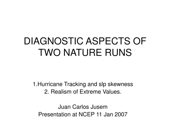
DIAGNOSTIC ASPECTS OF TWO NATURE RUNS 1.Hurricane Tracking and slp skewness 2. Realism of Extreme Values. Juan Carlos Jusem Presentation at NCEP 11 Jan 2007
Acknowledgements • The author has been benefited from discussions with Mr.Joseph Terry and Dr.Oreste Reale.
TWO NATURE RUNS • Material from two nature runs are to be presented: • GEOS-4 Finite Volume GCM, Sep 2004. • EC: Summer 2005.
GEOS-4 Finite Volume GCM • Terrain-following Lagrangian control volume vertical discretization of the conservation laws of mass momentum and energy. • Vertical Resolution: 32 levels. • Horizontal Resolution: 0.25 deg lat x 0.36 deg lon. • 2 D horizontal flux form semi-Lagrangian discretization.
Hurricane tracking and monthly skewness of sea level pressure • The skewness coefficient is the 3rd central moment of the normalized values of a statistical variable. • It is a measure of the asymmetry of a statistical distribution. • In the tropics, any ‘trough” axis of the contours of slp-skewness is co-located with a cyclone track.
Representation of a hurricane track (red line) by the axis of the negative monthly slp-skewness (green contours) ridge.(The monthly time series of slp for the points S, T, U are plotted in the next slide)
Comparing slp time-series of the “track point” T (red curve) and two points adjacent to the track.
SLP-skewness over the globe: not only hurricanes but also higher latitude “bombs” are captured.
Signatures of hurricane tracks appear in monthly variability (standard deviation) maps.
Time-series comparison between a hurricane track point (red curve, sk=-3.25) and a point of high variability in the storm track of the SH (black curve, sk=-0.47).
Same as previous slide,but with the time series normalized. (The spike-like nature of the more asymmetric (red) time series is kept in the normalized data)
Frequency distribution comparison between the hurricane track point (red, sk=-3.25, look at the long tail) and the point of high variability in the storm track of the SH (black, sk=-0.47)
In general, time series of slp at a hurricane track point can be approximmated by the gaussian function p(t) = A exp (-alpha * (t-tm)^2), in the vecinity of the time of min slp. In this case, alpha = 0.8
Conclusions • The horizontal pattern of sea level pressure skewness constitutes an excellent tool for having a FIRST LOOK of the set of hurricane trajectories during a month (or perhaps a season). • A track is marked by the axis of a “trough” in the horizontal distribution of slp-skewness. • In the extratropics, there is no correspondence between cyclone tracks and “troughs” in the slp-skewness pattern. But a significant value of skewness is indicative of an anomalous weather event. • Monthly slp-standard deviation patterns give a good hint of hurricane trajectories, but these trajectories do not appear as separate entities, like in the skewness pattern.
Assessment of the Realism of Extreme Values • Purpose: For a given variable, to assess the likelihood of values simulated by the nature run that are outside the range of observed values in the real world. • “Observed” means: produced by the NCEP-NCAR Reanalysis in the interval between the years 1948 and 2004. • Chosen Variable: 500 hPa monthly averaged geopotential (in what follows, z500), • Method: Comparison between the area covered by the out-of-range nature run values and the area covered by real world record-breaking-values, for the same month. The “range” for each grid point is the difference between the Reanalysis maximum and minimum for the grid point during the period 1948-2004. • Normalization: The chosen variable is normalized by multiplying by 100 the ratio between the difference of the variable and its minimum and the variable-range during the reanalysis interval 1948-2004. • The normalization is inspired in the centigrade scale. Normalized values greater than 100 (smaller than zero) represent z500 values greater (smaller) than any value ever observed at the same grid point.
Nature Run Average of 500 hPa Geopotential and Normalized Values.
Reanalysis September 2004 Average of 500 hPa Geopotential and Normalized Values.
Comparison between the area covered by nature run out-of-range values and Reanalysis record breaking values. • The comparison starts at 1978. • The period 1948-1977 has been used as the minimum period over which the expression “record breaking” is meaningful. • A record breaking takes place at a given grid point in September 1994 (say) if the Reanalysis z500 is greater or smaller that any “observed” z500 at the same grid point during the period 1948-1973 for September.
Comparison between the Area Covered by Record Breaking Values Each Year and the Area Covered by the Nature Run Out-of-Range Values.
CONCLUSION • Simple inspection of the previous slide suggests that the NATURE RUN is not an outlier, as far as monthly average of 500 hPa geopotential is concerned. • Of course, this is an exercise and z500 has been used to illustrate a methodology. We plan to apply the same methodology to other variables (like precip) whose realism might be challenged and for which, alternative verification datasets could be necessary.