Download
1 / 29
290 likes | 438 Views
Univariate Statistics Analyzing One Variable at a Time. 1. Chi Square 2. Kendall’s W Chi- squareTest 3. T-test for one mean. Chi-Square Goodness of Fit. When to use: number of variables analyzed ________ scaling of variable _________ Basic idea:

E N D
Univariate StatisticsAnalyzing One Variable at a Time 1. Chi Square 2. Kendall’s W Chi-squareTest 3. T-test for one mean
Chi-Square Goodness of Fit When to use: number of variables analyzed ________ scaling of variable _________ Basic idea: could the numbers you get (the observed value) come from a population which has the pattern I expect? (the expected value) Does the observed pattern of frequencies correspond to the expected pattern
The Chi Square Goodness of Fit Hypotheses • Ho: This sample could have come from a population that has this pattern:________________________________________________________________________________________________ • Ha: There is a different pattern in the sample than expected.
Chi-Square Goodness of Fit Chi-square calculated= sum of (Observedi -Expected i ) 2 Expected i degrees of freedom = number of resp. cat. -1 Alpha Value Critical Value
Now Graph chi-square calculated chi-square critical
Chi-Square Goodness of Fit What type of frozen dairy treat do you like best? 1. hard scoop ice cream 2. soft serve ice cream 3. chocolate covered ice cream bars Ho: Ha: Chi-square Calculated: Degrees of Freedom: Chi-square Critical: Graph
Chi-square Goodness of Fit Rules If the p-value is less than the alpha value, then _______ Ho; conclude the pattern in the data is NOT what you expected or wanted. If the p-value is greater than the alpha value, then _______ Ho; conclude, the pattern IS what you expected or wanted.
Do It Yourself Using SPSS -- What is the pattern for the favorite brand of soda? Ho: Ha:
Do It Yourself Using SPSS --(cont.) Degrees of Freedom: Chi-square Calculated: Chi-square Critical: Graph Conclusion:
Another Example What is the pattern for the number of people who drink a soda with breakfast? Ho: Ha:
Kendall’s W Chi-SquareTest • When to use: • number of variables ________ • scaling of variable ________ • Basic idea: compare the observed value (________________) with the values you would expect if NO PREFERENCE was shown in the data
The Kendall’s W Chi-square Test Hypotheses • Ho: There is no ranking in the data--there is no preference. • Ha: There is ranking in the data--there is preference, specifically, ______________________. • Chi-Square calculated: • sum of (Observedi -Expectedi)2Expectedi
Kendall’s W Chi-Square test First, multiply the rank-order data for each variable Variable 1 score = 1 (___) + 2 (___) +3 (___) ... Variable 2 score = 1 (___) + 2 (___) +3 (___) ... Variable 3 score = 1 (___) + 2 (___) +3 (___) ... Compute expected value Add up the total scores and divide by the number of variables
Example Ranking of movies: Pirates of the Caribbean, Shrek, Wall-E (n=20) Pirates Shrek Wall-E 1 10 7 3 2 4 8 8 3 6 5 9 Pirates = 1 (___) + 2 (___) +3 (___) = Shrek = 1 (___) + 2 (___) +3 (___) = Wall-E = 1 (___) + 2 (___) +3 (___) = Expected value:
Kendall’s W Chi-Square Test Degrees of freedom Alpha level Accept or reject Ho:
Rules If the p-value is greater than alpha, then _______ Ho, conclude that there no preference in the data. If the p value is less than alpha, then ___________ Ho. EXAMINE THE DATA TO DETERMINE PREFERENCE. (It may not be what you hypothesized!)
Do This With the Soda Rankings Ho: Ha: Rank calculations Expected value
Do This With the Soda Rankings (continued) Graph: Conclusion: reject or do not reject Ho Managerial implication
T-test for One Mean When to use: number of variables __________ scaling of variables __________ Basic idea Look at the confidence intervals. Any numbers in the same confidence intervals are considered the same. Key question--If my sample mean (xbar) is ___, can my population mean (mu) be ___?
Example Ho and Ha Ho: × = µ Ha: × ≠ µ (two-tailed test) Ho: X ≥ µ Ha: X < µ (one-tailed test – lower tail) Ho: X ≤ µ Ha: X > µ (one-tailed test – upper tail)
Hypotheses for T-test for One Mean Interested in the average number of sodas drunk per day to determine whether to install a new vending machine. Ho: The opposite of Ha: The population mean is equal or (less than/greater than) the number hypothesized. Ha: What you need to be actionable. The population mean is (less than/ greater than/ not equal to…) _____. Note: it is easier to write Ha first.
Calculations T calculated = x – µ Sx Where: X = sample mean µ = hypothesized population mean Sx =standard error
More T Calculations Degrees of freedom= n-1 Alpha level= T-critical value =
Now Graph t-calculated and t-critical value on a normal curve
Rules for T-test for One Mean If the calculated t-value is in the hump, ________ Ho. Conclude that your Ha is not correct. If the calculated t-value is in the tail then _____ Ho.
Practice Once Ho: Ha: The populations purchase intention for a gumball machine is >4. X-Bar: 4.5 SE= 0.15, n=60 T-calculated Degrees of freedom T-table Graph Conclusion: Reject or Do not Reject Ho Managerial implication:
Let’s go back to the previous example • Interested in the average number of sodas drunk per day to determine whether to install a new vending machine. • Ho: • Ha: • T-calculated • Degrees of freedom • T-table • Graph • Conclusion: Reject or Do not Reject Ho • Managerial implication
Now Use SPSS Ho: Ha: The average population rating for Coke when consumers know it is Coke is >6. T-calculated Degrees of freedom T-table Graph Conclusion: Reject or Do not Reject Ho Managerial implication:
Now Use SPSS • Ho: • Ha: The average population rating for Coke when consumers do not know it is Coke is < 5. • T-calculated • Degrees of freedom • T-table • Graph • Conclusion: Reject or Do not Reject Ho • Managerial implication: