A GPU Accelerated Explicit Finite-volume Euler Equation Solver with Ghost-cell Approach
360 likes | 539 Views
Session: Supercomputer/GPU and Algorithms (GPU-2). A GPU Accelerated Explicit Finite-volume Euler Equation Solver with Ghost-cell Approach. F.-A. Kuo 1,2 , M.R. Smith 3 , and J.-S. Wu 1* 1 Department of Mechanical Engineering National Chiao Tung University Hsinchu , Taiwan

A GPU Accelerated Explicit Finite-volume Euler Equation Solver with Ghost-cell Approach
E N D
Presentation Transcript
Session: Supercomputer/GPU and Algorithms (GPU-2) A GPU Accelerated Explicit Finite-volume Euler Equation Solver with Ghost-cell Approach F.-A. Kuo1,2, M.R. Smith3, and J.-S. Wu1* 1Department of Mechanical Engineering National Chiao Tung University Hsinchu, Taiwan 2National Center for High-Performance Computing, NARL Hsinchu, Taiwan 3Department of Mechanical Engineering National Cheng Kung University Tainan, Taiwan *E-mail: chongsin@faculty.nctu.edu.tw 2013 IWCSE Taipei, Taiwan October 14-17, 2013
Outline • Background & Motivation • Objectives • Split HLL (SHLL) Scheme • Cubic-Spline Immersed Boundary Method (IBM) • Results & Discussion • Parallel Performance • Demonstrations • Conclusion and Future work 2
Parallel CFD • Computational fluid dynamics (CFD) has played an important role in accelerating the progress of aerospace/space and other technologies. • For several challenging 3D flow problems, parallel computing of CFDbceomes necessary to greatly shorten the very lengthy computational time. • Parallel computing of CFD has evolved from SIMD type vectorized processing to SPMD type distributed-memory processing for the past 2 decades, mainly because of the much lower cost for H/W of the latter and easier programming. 4
SIMD vs. SPMD • SIMD (Single instruction, multiple data), which is a class of parallel computers, performs the same operation on multiple data points at the instruction level simultaneously. • SSE/AVX instructions in CPU and GPU computation, e.g., CUDA. • SPMD (Single program, multiple data) is a higher level abstraction where programs are run across multiple processors and operate on different subsets of the data. • Message passing programming on distributed memory computer architectures, e.g., MPI. 5
MPI vs. CUDA • Most well-known parallel CFD codes adopt SPMD parallelism using MPI. • e.g., Fluent (Ansys), CFL3D (NASA), to name a few. • Recently, because of the potentially very highC/P ratio by using graphics processor units (GPUs), parallelization of CFD code using GPUs has become an active research area based on CUDA, developed by Nvidia. • However, redesign of the numerical scheme may be necessary to take full advantage of the GPU architecture. 6
Split HLL Scheme on GPUs • Split Harten-Lax-van Leer (SHLL) scheme (Kuoet al., 2011) • a highly local numerical scheme, modified from the original HLL scheme • Cartesian grid • ~ 60 times of speedup (Nvidia C1060 GPU vs. Intel X5472 Xeon CPU) with explicit implementation • However, it is difficult to treat objects with complex geometry accurately, especially for high-speed gas flow. One example is given in the next page. • Thus, how to take advantage of easy implementation of Cartesian grid on GPUs, while improving the capability of treating objects with complex geometry becomes important in further extending the applicability of SHLL scheme in CFD simulations. 7
Staircase-like vs. IBM Staircase-like IBM Shock direction • Spurious waves are often generated using staircase-like solid surface for high-speed gas flows. 8
Immersed Boundary Method • Immersed boundary method (IBM) (Peskin, 1972; Mittal & Iaccarino, 2005 ) • easy treatment of objects with complex geometry on a Cartesian grid • grid computation near the objects become automatic or very easy • easy treatment of moving objects in computational domain w/o remeshing • Major idea of IBM is simply to enforce the B.C.’s at computational grid points thru interpolation among fluid grid and B.C.’s at solid boundaries. • Stencil of IBM operation is local in general. • Enabling an efficient use of original numerical scheme, e.g., SHLL • Easy parallel implementation 9
Objectives 10
Goals • To develop and validate an explicit cell-centered finite-volume solver for solving Euler equation, based on SHLL scheme, on a Cartesian grid with cubic-spline IBM on multiple GPUs • To study the parallel performance of the code on single and multiple GPUs • To demonstrate the capability of the code with several applications 11
SHLL Scheme - 1 Introduce local approximations Original HLL Final form (SHLL) is a highly local scheme i-1 i i+1 • New SR & SL term are approximated w/o involving the neighbor-cell data. • A highly local flux computational scheme: great for GPU! +Flux - Flux SIMD model for 2D flux computation 13
SHLL Scheme - 2 • Flux computation is perfectfor GPU application. • Almost the same as the vector addition case. • > 60 timesspeedup possible using a single Tesla C1060 GPU device. Performance compares to single thread of a high-performance CPU (Intel Xeon X5472) i-1 i i+1 Final Form (SHLL) +Flux - Flux SIMD model for 2D flux computation 14
Two Critical Issues of IBM • How to approximate solid boundaries? • Local Cubic Spline for reconstructing solid boundaries w/ much fewer points • Easier calculation of surface normal/tangent • How to apply IBM in a cell-centered FVM framework? • Ghost-cell approach • Obtain ghost cell properties by the interpolation of data among neighboring fluid cells • Enforce BCs at solid boundaries to ghost cells through data mapping from image points 16
Cell Identification Solid boundary curve Fluid cell Solid cell Ghost cell Define a cubic-spline function for each segment of boundary data to best fit solid boundary geometry Identify all the solid cells, fluid cells and ghost points Locate image points corresponding to ghost cells
Cubic-Spline Reconstruction (Solid Boundary) • The cubic spline method provides the advantages including : • A high order curve fitting boundary • Find these ghost cells easily. • Calculate the normal vector which is normal to the body surface. 18
BCs of Euler Eqns. Approximated form unit normal of body surface 19
IBM Procedures • Approximate the properties of the image points using bi-linear interpolation among neighboring fluid cells Interpolation Fluid cell Image point Solid cell Ghost point
Nearly All-Device Computation Start Set GPU device ID and flowtime Initialize T > flowtime Flux calculation True State calculation flowtime += dt False IBM Output the result CFL calculation Host 22 Device
Parallel Performance - 1 • Also named as “Schardin’s problem” • Test Conditions • Moving shock w/ Mach 1.5 • Resolution: 2000x2000 cells • CFLmax=0.2 • Physical time:0.35 sec. for 9843 time- steps using one GPU L=1 H=1 Moving shock x0.2 @ t=0 24
Parallel Performance - 2 Sec. Speedup • Resolution • 2000x2000 cells • GPU cluster • GPU: Geforce GTX590 (2x 512 cores, 1.2 Ghz3GB DDR5) • CPU: Intel Xeon X5472 • Overhead w/ IBM • 3% only • Speedup • GPU/CPU: ~ 60x • GPU/GPU: 1.9 @2 GPUs • GPU/GPU: 3.6 @4 GPUs 25
Shock over a finite wedge - 1 w/o IBM • In the case of 400x400 cells w/o IBM, the staircase solid boundary generates spurious waves, which destroys the accuracy of the surface properties. • By comparison, the case w/ IBM shows much more improvement for the surface properties. w/ IBM 27
Shock over a finite wedge - 2 Density contour comparison with IBM w/o IBM 28 t= 0.35 s • All important physical phenomena are well captured by the solver with IBM without spurious wave generation.
Transonic Flow past a NACA Airfoil Staircase boundary w/o IBM IBM result pressure pressure In the left case, the spurious waves appear near the solid boundary, but in the right case, we modify the boundary by using the IBM.
Transonic Flow past a NACA Airfoil Distribution of pressure around the surface of the airfoil Upper surf. Lower surf. Ghost cell method, J. Liu et al., 2009 New approach method These 2 results are very closed, and the right result is made by Liu in 2009, and the left result is made by the cubic spline IBM.
Transonic Flow past a NACA Airfoil Top-side shock wave comparison Furmanek*, 2008 New approach method * PetrFurmánek, “Numerical Solution of Steady and Unsteady Compressible Flow”, Czech Technical University in Prague, 2008
Transonic Flow past a NACA Airfoil Bottom-side shock wave comparison New approach method Furmanek*, 2008 * PetrFurmánek, “Numerical Solution of Steady and Unsteady Compressible Flow”, Czech Technical University in Prague, 2008
Summary • A cell-centered 2-D finite-volume solver for the inviscid Euler equation, which can easily treat objects with complex geometry on a Cartesian grid by using the cubic-spline IBM on multiple GPUs, is completed and validated • The addition of cubic-spline IBM only increase 3% of the computational time, which is negligible. • Speedup for GPU/CPU generally exceeds 60 times on a single GPU (Nvidia, Telsa C1060) as compared to that on a single thread of an Intel X5472 Xeon CPU. • Speedup for GPUs/GPUreaches 3.6 at 4 GPUs (GeForce) for a simulation w/ 2000x2000 cells.
Future Work • To modify the Cartesian grid to the adaptive mesh grid. • To simulate the moving boundary problem and real-life problems with this immersed boundary method • To change the SHLL solver to the true-direction finite volume solver, likes QDS