Download
1 / 20
200 likes | 297 Views
This comprehensive method involves vertical and horizontal tracking for particle analysis, focusing on wire calculations, trajectory estimations, angle predictions, and vertex constructions.

E N D
NKS Vertical Tracking( and etc)written at 2007/08/15 Tohoku Univ. Kyo Tsukada
Method • More than three hits of four stereo wires are required. • Two z candidates, z1 and z2, are found by the horizontal trajectory. • The relation, z=a+bx, is assumed in local coordinate. • From the least c2 method, most probably track is selected in 2^(numofstereohits) tracks.
Analyzer (1) • DCAnalysis::TrackSearch() • Horizontal tracking • SDC1,2,3, CDC4,5,8,9,12,13 are used. • DCAnalysis::VerticalTrackSearch() • Vertical tracking • CDC6,7,10,11 are used. • Z information of vertical wires are calculated from vertical tracking. • PTrack::calcObservables() • Calculating the Time of flight, flight length, b, mass, and so on. • The vertical angle of the track is estimated. The priority is as follows, • Result of PTrack::calcVerticalTrack(). • Z-information of OH as outer-side and the origin as other side.
Analyzer (2) • PTrack::calcVerticalTrack() • Vertical tracking • CDC6,7,10,11, IH and OH are used. • z1 and z2 are already found in DCTrack::VerticalTrackSearch(). • dz of IH and OHH ~ zlen/sqrt(12), OHV ~ 2cm • Z information of vertical wires are estimated from vertical tracking. • ParticleAnalysis::SetTimeZeroCorrection(…) • Correcting the Time of DC by • Time of IH associated a track • Time difference between slow particle and electron. • Tracking and vertical tracking again. • PVertex3D::ConstructVertex() • Constructing a vertex from 3D tracjectories.
Search Nearest Hit • For the killed layer method, DCTrack::SearchNearestHit is important. • Now, it can work even for stereo layers. • We can also get the drift length calculated from trajectory position. • We can derive the X-T curve of stereo layers.
X-T curves (before adjusting) run1150 Stereo Layers
X-T curves (after adjusting) run1150 Stereo Layers
Resolutions of January data • 915.param : run915 • 908-925.param : run917 • 929-952.param : run940 • 956-968.param : run960 • 972-991.param : run981 • 992-1017.param : run 1006 • 1022-147.param : run1036 • 1051-1071.param : run1065 • 1075-1097.param : run1085 • 1101-1122.param : run1112 • Right figures show the mean and sigma of gaussian fits for the run used to adjust parameters.
Resolutions of all run • Bottom figures show the mean and sigma of gaussian fits for all run. • The time dependence of sigmas are reasonable because of the lack of the chamber gas at the beginning of the experiment. • The mean of the residual is good only for the run used to adjust parameters. • At least, the offset parameters should be corrected run by run.
Plane efficiencies of January data • Bottom figures show the efficiencies for the run used to adjust parameters. • The efficiencies are estimated in the range, 20degree<| angle |. • Right bottom figures are the efficiencies with the distance cut, distance < 1.5*cellsize.
Vertical angular resolution (1) z@OHVL2 from OH z@OHVL2 from OH w/EV z@OHVL2 from DC z@OHVL2 from DC w/EV Run1128-1157 z@OHVL6 from OH z@OHVL6 from OH w/EV z@OHVL6 from DC z@OHVL6 from DC w/EV -0.9 < cosOA < 0.8 z@OHVL2 from OH z@OHVL2 from OH w/EV z@OHVL2 from DC z@OHVL2 from DC w/EV The bump due to EV is clearly seen. z@OHVL6 from OH z@OHVL6 from OH w/EV z@OHVL6 from DC z@OHVL6 from DC w/EV
Vertical angular resolution (2) -0.9 < cosOA < 0.8 Run1128-1157
Vertical angular resolution (3) Run1128-1157 • Vertical distribution for each OH w/ EV. • For OHVL4 and OHVR4, the correspondence between OH and EV are wrong.
Vertical angular resolution (4) Run1128-1157 • By taking the difference of adjacent bins, the resolutions are estimated. • The shadow of EV and the edges of OH are used.
Vertical angular resolution (5) Run1128-1157 • The positions of the edges of EV and the vertex resolutions are estimated. • The width of EV is 5 cm. • From tracking, the widths seems to be little narrow (?). • The sigma is less than 1 cm. Right Left
Vertical angular resolution (6) Run1128-1157 • The positions of the edges of OH and the vertex resolutions are estimated. • The height of OHV is 74.8 cm. • From tracking, the heights seems to be little small (?). • The sigma is about 1 cm. Right Left
Vertical angular resolution (7) Run1128-1157 • The positions of the edges of OH and the vertex resolutions are estimated. • Because the distribution is not flat, the fittings are done for one side of each OH. • From tracking, the heights seems to be little low (?). • The sigma is about 1-2 cm.
Vertex resolutions in 3D • Vertex resolution • The dx is estimated by the difference of the distribution. • I could not find how to estimate the dy and dz. • Right figures show the vertex distributions in target. • If the beam size is negligible, this distributions give dy and dz. Run1150 Run1128-1157
Resolution of Vertical angle • The vertical resolution at target is about 2 mm. • The vertical resolution at OH is about 10 mm. • The radius of OH from origin is typically 120 cm. The angular resolution (dq) is about 8.5 mrad.
Summary • The vertical tracking works well. • For DC tracking, the time information of IH and OH are used. • The plane resolutions are about 500 um for CDC and 300 um for SDC. These values include the tracking resolution. • We should adjust the drift parameters run by run. • The plane efficiency are more than 98% in stable runs. But, in this study, the efficiencies in the forward region are not estimated. • The vertical position resolutions are about 10mm@OH and 2mm@target. • The vertical angular resolution is about 8.5 mrad. • The z-position of the vertex point can be calculated.