Download
1 / 28
280 likes | 346 Views
This research focuses on setting due dates in complex product systems with uncertain processing times. It includes an overview, literature review, lead time distribution estimation, due date planning, industrial case study, discussion, conclusion, and future work. The study discusses the challenges of uncertainty in processing, presents two research streams, limitations of existing methods, analytical results, lead time distribution estimation, industrial case study parameters, due date simulation, and methods for setting due dates.

E N D
Due Date Planning for Complex Product Systemswith Uncertain Processing Times By: Dongping Song Supervisor: Dr. C.HicksandDr. C.F.Earl Dept. of MMM Eng. Univ. of Newcastle upon Tyne April, 1999
Overview 1. Introduction 2. Literature review 3. Leadtime distribution estimation 4. Due date planning 5. Industrial case study 6. Discussion and conclusion 7. Further work
Uncertainty in processing • disrupt the timing of material receipt • result in deviation of completion time from due date
Introduction • Complex product system • Assembly and product structure • Uncertain processing times • Cumulative and interacting • Problem : setting due date in complex product systems withuncertainprocessing times
Literature Review Two principal research streams [Cheng(1989), Lawrence(1995)] • Empirical method: based on job characteristics and shop status. Such as: TWK, SLK, NOP, JIQ, JIS Due date(DD) = k1×TWK + k2 • Analytic method: queuing networks, mathematical programming etc.by minimising a cost function
Literature Review Limitation of above research • Both focus on job shop situations • Empirical - rely on simulation, time consuming in stochastic systems • Analytic - limited to “small” problems
Simple Two Stage System • Product structure
Planned start time S1, S1i • Holding cost at subsequent stage • Resource capacity limitation • Reduce variability
Minimum processing time M1 • Prob. density func.(PDF)Cumul. distr. func.(CDF) • Big variance may result in negative operation times
Analytical Result • CDF of leadtime W is: FW(t)= 0, t<M1+S1; FW(t) = F1(M1) FZ(t-M1) + F1¢ÄFZ, t ³ M1 + S1. where F1 ¾ CDF of assembly processing time; FZ¾ CDF of actual assembly start time; FZ(t)= P1n F1i(t-S1i) ľ convolution operator in [M1, t - S1]; F1¢ÄFZ= òF1¢(x) FZ(x-t)dx
Leadtime Distribution Estimation Complex product structure • approximate method Assumptions • normally distributed processing times • approximate leadtime by truncated normal distribution (Soroush, 1999)
Leadtime Distribution Estimation Normal distribution approximation • Compute mean and variance of assembly start time Z and assembly process time Q : mZ, sZ2andmQ, sQ2 • Obtain mean and variance of leadtime W(=Z+Q): mW = mQ+mZ, sW2 = sQ2+sZ2 • Approximate W by truncated normal distribution: N(mW, sW2), t ³ M1+ S1. More moments are needed if using general distribution to approximate
Due Date Planning • Achieve a specified probability ÞDD* by N(0, 1)
Due Date Planning • Mean absolute lateness (MAL) ÞDD* = median • Standard deviation lateness (SDL) ÞDD* = mean • Asymmetric earliness and tardiness cost ÞDD* by root finding method
Industrial Case Study • Product structure 17 components 17 components
System parameters setting • normal processing times • at stage 6: m =7days for 32 components, m =3.5 days for the other two. • at other stages : m=28 days • standard deviation: s= 0.1m • backward scheduling based on mean data • planned start time: 0 for 32 components and 3.5 for other two.
Product Due Date • Simulation verification for product due date to achieve specified probability
Stage Due Dates • Simulation verification for stage due dates to achieve 90% probability
Discussion • Minimum processing time • Production plan • Stage due date
Conclusion • Complex product systems with uncertainty • A procedure to estimate leadtime distribution • Approximate method to set due dates • Used to design planned start times
Further Work • Skewed processing times • Using more general distribution to approximate, like l-type distribution • Resource constraint systems