Download
1 / 32
320 likes | 502 Views
Uncertain Observation Times. Shaunak Chatterjee & Stuart Russell Computer Science Division University of California, Berkeley. Overview. Why uncertain observation times matter Scenarios considered: Each event is observed: Efficient DP algorithm Missing and false events:

E N D
Uncertain Observation Times ShaunakChatterjee & Stuart Russell Computer Science Division University of California, Berkeley
Overview • Why uncertain observation times matter • Scenarios considered: • Each event is observed: • Efficient DP algorithm • Missing and false events: • Practical approximation algorithm 3. Multiple asynchronous observation streams
Motivation • Two types of data streams • Automatically time-stamped data traces • Human annotations for temporal events • Many essential facts cannot be recorded automatically • Human-generated timestamps often wrong • Assuming the correctness of timestamps can lead to nonsense results
Example: at 16.30, nurse enters “gave phenylephrine at 16.00” Event timestamp Data entry time
Example: at 16.30, nurse enters “gave phenylephrine at 16.00” Actual event time Data entry time
Ubiquity of uncertain observation times • Nurse monitoring a patient in the ICU • Hundreds of events recorded by the nurse • Usually recorded after event, sometimes before • Manual recording of events • Science experiments • Biology, chemistry, physics • Industrial plants • Multiple observation traces • Various historians’ accounts of a period • Only one underlying truth
Sample trace generated from model • Correct chronological ordering of time stamps Time Actual time of event (ai) Recorded time of event (mi) Recording time of event (di) Nurse gives medicine at 10:23 a.m. Nurse records event at 11:00 a.m. Previous event’s time stamp (10:15 a.m.) Nurse records time of event as 10:30 a.m.
Dynamic Bayesian networks • DBNs are discrete-time multivariate stochastic process models (include HMMs and KFs) • DBNs facilitate modeling of complex systems with sensor noise etc. Large-scale physiological models pursued since the 1960s, but little attention paid to nature of real data
Simple DBN representation Y1 Y2 Y3 Y4 Y5 Y6 Y7 Y8 true false true true false false false false X6 X1 X2 X3 X4 X5 X7 X8 5 7 2 a1 a2 a3 4 8 2 m1 m2 m3 8 6 6 d1 d2 d3
Objective • To design a graphical model that allows for uncertainty in observation times • Derive efficient inference algorithms • Naïve algorithm has O(MT) complexity • Reduce to O(MT) • Ordering constraints • Dynamic programming
Key constraint assumption • Person recording events gets the order right • Valid association • Invalid association • For all i, j: mi > mj => ai > aj Time Actual time of event (ai) Recorded time of event (mi) Time Actual time of event (ai) Recorded time of event (mi)
Pre-computation step • Likelihood of the data segment between the current event time stamp (ak) and the next hypothesized event time stamp (ak+1) • Pre-compute for all k, and all possible values of ak and ak+1
Complexity • Modified time complexity O(MS2T) • M: maximum size of the time window of uncertainty • S: # states in system • T: number of time steps • Space complexity • O(KM2) – storing • O(KM) – storing α, β and γ
Simulation results – Increased likelihood of evidence Window of uncertainty
Simulation results – Computation time vs size of uncertainty window
Unreported events, false reports • Not all events are reported • Unobserved • Negligence • Not all reports are true • Double entry of a single data point • Misinterpretation of information • Intended actions reported but not carried out
Missing and false reports θ2 θ1 θ3 θ4 Event i reported? (θi) a1 a2 a3 a4 Actual time of event (ai) Φ1 Φ2 Φ3 Index of event corresponding to report j (φi) Recorded time of event (mi) m1 m2 m3
Modified DP and complexity • The previous algorithm was compact because of the one-to-one correspondence between events and reports • Now have to consider all possibilities • Unless there are constraints (more on this later) • Chronological mapping of events’ time stamps still holds • This again leads to an efficient dynamic program
Computational complexity • In the general case, uncertainty windows are no longer limited, since event i can be associated with any report j • O(IJT2) • I is the number of hypothesized events • J is the number of reports • T is the length of the temporal sequence
Practical assumptions – I • Data entries are made in blocks • All reports in a given block (e.g., the night shift) must be for events that occurred (really or otherwise) in that block • Computational complexity is linear in T if blocks are of constant size
Practical assumptions – II • When unobserved events and false reports are both rare events • We can perform approximate inference by NOTconsidering all possible aimjassociations • The posterior distribution is highly concentrated along the “skewed diagonal” corresponding to a small number of errors • Assuming a bounded number of errors gives time complexity proportional to T
Simulation results – Posterior is peaked around the skewed diagonal
Simulation results – Hypothesizing more events leads to better recall
Multiple observation sequences • Formulation • Several “sources” reporting on the same events • Key assumption • Individual report sequences are independent given the actual truth (the X chain)
θi+1 θi θI Latent trajectory ai ai+1 aI Φj(1) Φj+1(1) ΦJ(1) Evidence trajectory 1 mj(1) mj+1(1) mJ(1) Φj(R) Φj+1(R) ΦJ(R) Evidence trajectory R mJ(R) mj(R) mj+1(R)
Multiple observation sequences • Formulation • Several “sources” reporting on the same events • Key assumption • Individual report sequences are independent given the actual truth (the X chain) • Inference • Similar DP algorithms apply, given the assumptions of ordering constraints, blocks, etc. • Complexity increases linearly with the number of report sequences
Conclusions • Handling uncertainty in observation times is critical for correct modeling and inference • Assumptions about qualitative accuracy (e.g., order of events) can be very helpful • Given such assumptions, the computational complexity of inference remains unchanged (modulo some constant factors) while handling the following cases • Noisy observation times • Missing and false reports • Multiple report sequences
Thank You! QUESTIONS?