Download
1 / 12
120 likes | 285 Views
CS100J 02 May Matlab and PI and other things. The notation j:k gives a row matrix consisting of the integers from j through k. >> 1:8 ans = 1 2 3 4 5 6 7 8 The notation j:b:k gives a row matrix consisting of the integers from j through k in steps of b.

E N D
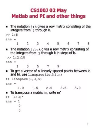
CS100J 02 May Matlab and PI and other things • The notation j:k gives a row matrix consisting of the integers from j through k. >> 1:8 ans = 1 2 3 4 5 6 7 8 • The notation j:b:k gives a row matrix consisting of the integers from j through k in steps of b. >> 1:2:10 ans = 1 3 5 7 9 • To get a vector of n linearly spaced points between lo and hi, use linspace(lo,hi,n) >> linspace(1,3,5) ans = 1.0 1.5 2.0 2.5 3.0 • To transpose a matrix m, write m’ >> (1:3)’ ans = 1 2 3
sum, prod, cumsum, cumprod • Function sum adds row elements, and function prod multiplies row elements: >> sum(1:1000) ans = 500500 >> prod(1:5) ans = 120 • Function cumsum computes a row of partial sums and cumprod computes a row of partial products: >> cumprod(1:7) ans = 1 2 6 24 120 720 5040 >> cumsum(odds) ans = 1 4 9 16 25 36 49 64
Compute Pi by Euler Formula • Leonard Euler (1707-1783) derived the following infinite sum expansion: 2/ 6 = 1/j 2 (for j from 1 to ) >> pi = sqrt( 6 .* cumsum(1 ./ (1:10) .^ 2)); >> plot(pi) • To define a function, select New/m-file and type definition: % = a vector of approximations to pi. function e = euler(n) e= sqrt( 6 .* cumsum(1 ./ (1:n) .^ 2)); • Select SaveAs and save to a file with the same name as the function. • To invoke: >> pi= euler(100); >> plot(pi)
Help System • Use on-line help system >> help function ... description of how to define functions ... >> help euler = a vector of approximations to pi, using Euler’s appoximation
Compute Pi by Wallis Formula • John Wallis (1616-1703) derived the following infinite sum expansion: (2*2) * (4*4) * (6*6) * ... / 2 = -------------------------- (1*3) * (3*5) * (5*7) * ... • Terms in Numerator evens .^ 2 • Terms in Denominator 1 3 5 7 9 ... odds 3 5 7 9 11 ... odds + 2 ----------------- 1*3 3*5 5*7 7*9 9*11 . . . i.e. odds .* (odds + 2) • Quotient prod( (evens .^ 2) ./ (odds .* (odds+2)) • Successive approximations to Pi pi = 2 .* cumprod( (evens.^2) ./ (odds .* (odds+2)) )
Wallis Function • Function Definition function w = wallis(n) % compute successive approx’s to pi. evens = 2 .* (1:n); odds = evens - 1; odds2 = odds .* (odds + 2); w = 2 .* cumprod( (evens .^ 2) ./ odds2 ); • Contrasting Wallis and Euler approximations >> plot(1:100, euler(100), 1:100, wallis(100))
Compute Pi by Throwing Darts • Throw random darts at a circle of radius 1 inscribed in a 2-by-2 square. • The fraction hitting the circle should be the ratio of the area of the circle to the area of the square: f = / 4 • This is called a Monte Carlo method y 1 x 1
Darts • (h,w) yields an h-by-w matrix of random numbers between 0 and 1. >> x = rand(1,10); >> y = rand(1,10); • Let d2 be the distance squared from the center of the circle. >> d2 = (x .^ 2) + (y .^ 2); • in be a row of 0’s and 1’s signifying whether the dart is in (1) or not in (0) the circle. Note 1 is used for true and 0 for false. >> in = d2 <= 1; • hits(i) be the number of darts in circle in i tries >> hits = cumsum(in); • f(i) be franction of darts in circle in i tries >> f = hits ./ (1:10); • pi be successive approximations to pi >> pi = 4 .* f;
Compute Pi by Throwing Needles • In 1777, Comte de Buffon published this method for computing : N needles of length 1 are thrown at random positions and random angles on a plate ruled by parallel lines distance 1 apart. The probability that a needle intersects one of the ruled lines is 2/. Thus, as N approaches infinity, the fraction of needles intersecting a ruled line approaches 2/.
Subscripting • Subscripts start at 1, not zero. >> a = [1 2 3; 4 5 6; 7 8 9] ans = 1 2 3 4 5 6 7 8 9 >> a(2,2) ans = 5 • A range of indices can be specified: >> a(1:2, 2:3) ans = 2 3 5 6 • A colon indicates all subscripts in range: >> a(:, 2:3) ans = 2 3 5 6 8 9
Control Structures: Conditionals ifexpression list-of-statements end ifexpression list-of-statements else list-of-statements end ifexpression list-of-statements elseifexpression list-of-statements . . . elseifexpression list-of-statements else list-of-statements end
Control Structures: Loops whileexpression list-of-statements end forvariable = lo:hi list-of-statements end forvariable = lo:by:hi list-of-statements end