Download
1 / 27
270 likes | 353 Views
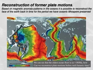
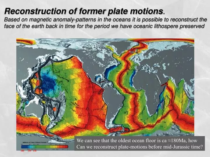
Reconstruction of former plate motions . Based on magnetic anomaly-patterns in the oceans it is possible to reconstruct the face of the earth back in time for the period we have oceanic lithospere preserved. We can see that the oldest ocean floor is ca ≈180Ma, how

E N D
Reconstruction of former plate motions. Based on magnetic anomaly-patterns in the oceans it is possible to reconstruct the face of the earth back in time for the period we have oceanic lithospere preserved We can see that the oldest ocean floor is ca ≈180Ma, how Can we reconstruct plate-motions before mid-Jurassic time? 180 155 130
We see that if magnetic anomalies in the oceans were the only basis for plate-reconstructions we would have no quantitative way of reconstructing older plate-configurations. Paleomagnetism is the only quantitative important method to produce older reconstructions (before present day ocean-floor mag anomalies) Preconditions for using paleomag: The earth’s magnetic poles coinside with the geographical poles over time. The magnetic field is vertical at the poles and horizontal at the equator, and the inclination (I) changes progressively with magnetic latitude () according to tan I = 2 tan . The earth’s magnetic field may be frozen-in as remanent magnetism in a rock, and the remanence may be preserved through geological time. A database of well-defined and well-dated magnetic remanences from various time periods for one defined area may be used to determine the same area’s position with respect toe the magnetic poles (or vice versa) for the periods for which we have well-defined remanences. Paleomagnetic remanence shows latitude and direction (azimuth) to a magnetic pole. Paleomagnetic data thus only give information on latitude and plate-velocity across latitude. Assumptions on paleo-longitude must be based on other criteria, such as a fixed point (hot-spot, fixed continent etc) for the time-period in question.
The magnetic field varies in orietation and intencity, but over geological time it coinsides with the geographical poles (rotation poles) Mag. pole positions thorugh the past 2000 yr And with the average shown.
The present-day total magnetic field (H) at a site is decomposed as shown in a vertical and horizontal component. These components give the Inclination and Declination of the total field. Normalized over time the declination will show The direction to the geograpical poles, and the inclination will be a function of latidtude.
A magnetic pole determined by paleomagnetism is defined by the average of poles from one area and from rocks with well-known ages. The magnetic pole is positioned on a great circle defined by the declination.
The magnetic pole will sit on a great circle definde by the declination. Uncertainty elipse
N-American poles fra mezo- og cenozoikum. Ages for poles and their 95% confidence is shown. Notice the dotted curve constructed through the uncertainty ellipses. 4 Mid-Cretaceous poles from 4 sites in N-America. If there is no qualitiative difference in the poles, the average of these poles will define the Mid- Cretaceous pole of N-America.
SUCH A BEST FIT CURVE IS KNOWN AS: ”APPARENT-POLAR-WANDER PATH” or APWP The APWP describes the relative motion of a continent to a pole or vice verca.
Principle for paleogeographical reconstruction by a APWP APWP for the plate M in the period 0 to 80 Ma is shown as a red curve
APWPs for N-America og Eurasia from the Ordovician to the Jurassic. N-America og Eurasia rotated back to the position before the N-Atlantic opened (Bullard fit) NOTICE THE COINCIDENCE OF THE APWPs FOR THE 2 CONTINENTS!
Paleomagnetism, methods and data quality: • keywords: • Curie temperature, Magnetite 5800C, Hematite 6800C • Thermal Remanent Magnetism (TRM), • Sediment Remanent Magnetism (SRM) • Thermo-chemical Remanent Magnetism (CRM), • Field tests: • Fold test • Conglomerate test • Contact test • Data quality: • Sampling and sample-handling • Thermal demagnetisation (thermal cleaning) • Alternating field demagnetisation • Instrument quality
Fold test Fold test Magnetization is older than the folding (positive fold test) Magnetization is younger than the folding (negativ folde test)
Conglomerate test Magnetization is close to arbitary in the pebbles and probably primary i.e. than the conglomerate (positive conglomerate test) Magnetization is parallel in the pebbles and probably secondary (negative conglomerate test)
Contact test The dyke has its own remanence, and remagnetizes the wall-rocks near the contact. A positive contact test indicating that magnetization is primary. The remanence in the dyke cannot be distinguished from the magnetization of the wall-rocks. A negative contact test.
Sample collection and handling Samples are drilled out in cores with non-magnetic equipment Samples are oriented accurately with compass and if possible sun-compass a
Handling, demag. in a room without a magnetic field Spinner- or supercondutive magnetometer Magnetic suseptibility Thermal demagnetization Alternationg field demag.
NMR WITH SEVERAL COMPONENTS b) Vertical plane a) Horizontal plane c) Horizontale og vertical projection into one vektor component figure.
NMR WITH TWO COMPONENTS, here shown in RED og BLUE The poles of both components can be determined, and if they are distinctly and statistically different we can assume that the magnetizations were formed at two different geographical locations! If the APWP is well determinded will the pole´s location on the APWP give information about the age of the magnetizations.
460 Ma 440 Ma 400 Ma 420 Ma 500 Ma Caledonian orogenic cycle in brief BALTICA a separate continent ≈ 550-425Ma Notice that traditional Wilson-cycle tectonics does not work to explain formation of the Caledonides http://www.geodynamics.no/platemotions/500-400/
OTHER APPLICATIONS OF PALMAG DATE EVENTS STUDY PALEOCLIMATE BELTS (SNOWBALL-EARTH HYPOTHESIS) ETC. HERE IS AN EXAMPLE:
CASE STUDY: LÆRDAL-GJENDE FAULT
CASE STUDY: LÆRDAL-GJENDE FAULT Breccias along a fault cutting all major tectonic units in south Norway, can we find the age of brecciation and therefore movement?
The results: Example of 2-component magnetization The components plotted in stereograms horizontal vertical
LGF-case study: The poles for the two magnetizations are plotted on the APWP for EURASIA. Vi can see that the comparison gives a Permian and late-Jurassic to Cretaceous age for the two components respectively. We interpret these to represent two stages of movement on the LGF
Reconstruction of former plate motions. Based on magnetic anomaly-patterns in the oceans it is possible to reconstruct the face of the earth back in time for the period we have oceanic lithospere preserved We can see that the oldest ocean floor is ca ≈180Ma, how Can we reconstruct plate-motions before mid-Jurassic time? 180 155 130