Download

1 / 44
450 likes | 592 Views
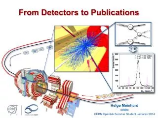
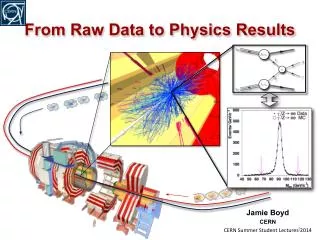
From Raw Data to Physics Results. Jamie Boyd CERN CERN Summer Student Lectures 2014. Outline. Summary Brief overview of the full lecture course A simple example Measuring the Z 0 cross-section Reconstruction & Simulation Track reconstruction Calorimeter reconstruction

E N D
From Raw Data to Physics Results Jamie Boyd CERN CERN Summer Student Lectures 2014
Outline • Summary • Brief overview of the full lecture course • A simple example • Measuring the Z0 cross-section • Reconstruction & Simulation • Track reconstruction • Calorimeter reconstruction • Physics object reconstruction • Simulation • Physics Analysis • Data Quality • Z’->ll • H->γγ • H->ZZ->4l • Computing infrastructure • The End! Fridays Lecture TodaysLecture • Disclaimer : Much of the content based on previous years lectures • Thanks to G. Dissertori
Reconstruction • Detector reconstruction • Tracking • finding path of charged particles through the detector • Calorimeter reconstruction • finding energy deposits in calorimeters from charged and neutral particles • Combined reconstruction • Electron/Photon identification • Muon identification • Jet finding • Calibrations and alignments applied at nearly every step
Important figures of merit for reconstructed objects • Efficiency • how often do we reconstruct the object – e.g. tracking efficiency Efficiency = (Number of Reconstructed Tracks) / (Number of True Tracks) Reconstructed track matched to true track!
Important figures of merit for reconstructed objects • Efficiency • how often do we reconstruct the object – e.g. tracking efficiency • Resolution • how accurately do we reconstruct it – e.g. energy resolution Electron energy resolution from simulation Energy resolution = (Measured_Energy – True_Energy)/ True_Energy
Important figures of merit for reconstructed objects • Efficiency • how often do we reconstruct the object – e.g. tracking efficiency • Resolution • how accurately do we reconstruct a quantity – e.g. energy resolution • Fake rate • how often we reconstruct a different object as the object we are interested in – e.g. a jet faking a electron Fake rate = (Number of jets reconstructed as an electron) / (Number of jets)
Important figures of merit for reconstructed objects • Efficiency • how often do we reconstruct the object – e.g. tracking efficiency • Resolution • how accurately do we reconstruct a quantity – e.g. energy resolution • Fake rate • how often we reconstruct a different object as the object we are interested in – e.g. a jet faking a electron These quantities depend on the detector, but also on the reconstruction and calibrations and alignment!
Important figures of merit for reconstructed objects • Efficiency • how often do we reconstruct the object – e.g. tracking efficiency • Resolution • how accurately do we reconstruct a quantity – e.g. energy resolution • Fake rate • how often we reconstruct a different object as the object we are interested in – e.g. a jet faking a electron For physics analysis it is important to have high efficiency, good resolution, and low fake rates to be able to measure the efficiencies, resolutions and fake rates and their uncertainties (not easy)
Reconstruction Goals • High efficiency • Good resolution • Low fake rate • Robust against detector problems • Noise • Dead regions of the detector • Be able to run within the computing resource limitations • CPU time per event • Memory use
Tracking • Track finding very important for analysis • Tracks are used directly in the reconstruction of • Electrons • Muons • And to a lesser extent in Tau, Jet and photon reconstruction • For reconstructed tracks we know • Momentum • straighter the track the higher momentum it is • Charge • Point of closest approach to the interaction point (important to identify particles such as b-quarks which have a long lifetime and so travel a measurable distance before they decay)
Quiz: Tracking by eye - Can you find the 50 GeV Track? cf Aaron Dominguez
Track Fitting • 1D straight line fit as simple case • Two perfect measurements • away from interaction point • no measurement uncertainty • just draw a straight line through them and extrapolate • Imperfect measurements give less precise results • the farther you extrapolate, the less you know Smaller errors and more points help to constrain the possibilities.But how to find the best point from a large set of points? • Quantitatively • parameterize a track: • In case of straight line or, eg., helix in case of magnetic field present • Find track parameters by Least-Squares-Minimization • Obtain also uncertainties on track parameters predicted track position at ith hit position of ith hit uncertainty of ith measurement
“Typical” size of errors 10 cm 10 cm ±10 microns ±10 microns • Error δd on position is about ±10 microns • Error δθ on angle is about ±0.1 milliradians (±0.002 degrees) • Satisfyingly small errors • allows separation of tracks that come from different particle decays (which can be separated at the order of mm) • Problem 1: • we “see” particles by interaction with a detector (=material) • interaction leads to : energy loss, change in direction • This is Multiple Scattering • Charged particles passing through matter “scatter” by a random angle • Need more sophisticated algorithms to be able to take this into account examples: 300 micron Si : RMS = 0.9 mrad /βp 1 mm Be : RMS = 0.8 mrad /βp ➔ leads to additional position errors
“Typical” size of errors 10 cm 10 cm ±10 microns ±10 microns • Error δd on position is about ±10 microns • Error δθ on angle is about ±0.1 milliradians (±0.002 degrees) • Satisfyingly small errors • allows separation of tracks that come from different particle decays (which can be separated at the order of mm) • Problem 2: • Tracking detector elements are not positioned in space with perfect accuracy • Can be misaligned with respect to each other by upto ~100 microns • Needs to be taken into account by the track finding software • Need to derive alignment corrections from the data and apply these in track reconstruction much exaggerated misalignment perfect alignment misaligned real detector
Tracker Alignment Worse alignment Improved alignment Simulation with perfect alignment - Improving the tracker alignment description in the reconstruction gives better track momentum resolution which leads to better mass resolution. - Can see the reconstructed Z width gets narrower if we use better alignment constants. Very important for physics analysis to have good alignment. - Alignment of detector elements can change with time for example when the detector is opened for repair, or when the magnetic field is turned on and off.
Answer: Tracking by eye - Can you find the 50 GeV Track? cf Aaron Dominguez
(aside) Pileup • When the LHC collides bunches of protons we can get more than one p-p interaction – this is called pileup • The number of pileup interactions depends on the LHC parameters • How many protons per bunch • How small the bunches have been squeezed • For last year we have on average ~20 interactions every time the bunches cross • These pileup interactions give lots of low momentum tracks • We can usually identify which tracks are from which interactions by combining tracks that come from the same vertex • Pileup can cause difficulties for some physics analyses • Also causes reconstruction to need more computing power • But allows us to get more luminosity 1011 protons 1011 protons beam 2 beam 1
Recent Z->μμ event in ATLAS. With 11 reconstructed vertices. Tracks with transverse momentum above 500MeV are shown (PT>0.5GeV). How can we do physics analysis with such a mess of tracks in the detector?
Recent Z->μμ event in ATLAS. With 11 reconstructed vertices. Tracks with transverse momentum above 2.0GeV are shown (PT>2.0GeV). How can we do physics analysis with such a mess of tracks in the detector?
Recent Z->μμ event in ATLAS. With 11 reconstructed vertices. Tracks with transverse momentum above 10GeV are shown (PT>10GeV). How can we do physics analysis with such a mess of tracks in the detector? By applying a cut on the object momentum the event becomes much cleaner and easier to analyze
Last displays were from early 2011 when average pileup was ~6 interaction / bunch crossing. Since then it has rapidly increased: Last year the average pileup was ~20! Lots of work has gone into making reconstruction robust against pileup. ie. making it so that efficiency/ resolution do not depend on amount of pileup
Goals • Reconstruct energy deposited by charged and neutral particles • Determine position of deposit, direction of incident particles • Be insensitive to noise and “un-wanted” (un-correlated) energy (pileup) CMS and obtain the best possibleresolution!
Clusters of energy • Calorimeters are segmented in cells • Typically a shower extends over several cells • Useful to reconstruct precisely the impact point from the “center-of-gravity” of the deposits in the various cells • Example CMS Crystal Calorimeter: • electron energy in central crystal ~ 80 %, in 5x5 matrix around it ~ 96 % • So task is : identify these clusters and reconstruct the energy they contain front view side view view in (φ,η) cells
Cluster Finding • Clusters of energy in a calorimeter are due to the original particles • Clustering algorithm groups individual channel energies • Don’t want to miss any; don’t want to pick up fakes Projection high threshold, for seed finding low threshold, against noise • Simple example of an algorithm • Scan for seed crystals = local energy maximum above a defined seed threshold • Starting from the seed position, adjacent crystals are examined, scanning first in φ and then in η • Along each scan line, crystals are added to the cluster if • 1. The crystal’s energy is above the noise level (lower threshold) • 2. The crystal has not been assigned to another cluster already
Difficulties • Careful tuning of thresholds needed • needs usually learning phase • adapt to noise conditions • too low : pick up too much unwanted energy • too high : loose too much of “real” energy. Corrections/Calibrations will be larger example : one lump or two? high threshold, for seed finding low threshold, against noise
Energy Calibration • Need to apply calibrations to the cell and cluster energies • Correct for energy lost before the calorimeter and for energy leaking out the back • Equalize the response across the detector (different parts of the detector can have different responses because of the way they are built etc..) • The purpose of the calibrations are to correct the measured energy to give as close as possible to the true energy of the incident particle • Calibration constants can be complex functions of the position and energy of the cluster • ECALIB = f(EMEASURED, η, ϕ, …) , f includes various calibration constants • Calibration very important to get the best energy resolution Electron energy resolution from simulation
Electron/Photon Identification • Electron/Photon reconstruction takes as input the tracks and calorimeter clusters already produced • Electron/Photon leave narrow clusters in the electromagnetic calorimeter • Apply selection on the cluster shape to reduce background from jets • Electron has track pointing at cluster • Requires aligning the calorimeter with the tracker • Photon has no track pointing at it • Final Electron momentum measurement can come from tracking or calorimeter information (or a combination of both) • Often have a final calibration to give the best electron energy • Often want isolated electrons • Require little calorimeter energy or tracks in the region around the electron
An electron in ATLAS 1. Narrow cluster in electromagnetic calorimeter 2. No energy in the hadronic calorimeter behind 2. High momentum track pointing at cluster
Electron/Photon Backgrounds • Hadronic jets leave energy in the calorimeter which can fake electrons or photons • Usually a Jet produces energy in the hadronic calorimeter as well as the electromagnetic calorimeter • Usually the calorimeter cluster is much wider for jets than for electrons/photons • So it should be easy to separate electrons from jets • However have many thousands more jets than electrons, so need the rate of jets faking an electron to be very small ~10-4 • Need complex identification algorithms to give the rejection whilst keeping a high efficiency Example of an electron energy deposit in the electromagnetic calorimeter in ATLAS. Use shower shape variables based on size of cluster in the radial and longitudinal directions to distinguish from hadronic showers (see next slide)
Electrons / Jets Electron/Photon Backgrounds Example of different calorimeter shower shape variables used to distinguish electron showers from jets in ATLAS
Muon identification CMS • Combine the muon segments found in the muon detector with tracks from the tracking detector • Momentum of muon determined from bending due to magnetic field in tracker and in muon system • Combine measurements to get best resolution • Need an accurate map of the magnetic field in the reconstruction software • Alignment of the muon detectors also very important to get best momentum resolution Muon segment in drift tubes
Simulation • Simulated data samples needed for • Designing experiments • Tuning analysis selections • Background estimation • Efficiency, resolution and fake-rate estimation • To get best physics outputs from the experiment it is essential to have an accurate simulation of the detector • Lots of work goes into tuning the simulation to give best description of the data • Test beam studies from construction period of the detector used to tune simulation (test beam allows to study detector response to known particle types and momenta – e.g. 20GeV electrons) • Very detailed simulation of the detector • Detailed description of the detector geometry • Accurate simulation of the detector electronics response • Include detector ‘noise’ in the simulation • Keep the ‘truth’ information • Allows efficiency, resolution and fake rates to be estimated
Simulation workflow Electronics Simulation Simulate the response of the detector elements to the ‘hits’ from the electron. Simulate the voltage pulse on the detector and how the detector electronics works. The output of this stage is very similar to the raw data from the detector. (but we keep the truth information). • Detector Simulation • Simulate the propagation of the electrons through the detector. • Including: • bending in the magnetic field • leaving hits in the tracking detector elements • interacting with the material in the detector • interacting in the calorimeter (detailed description of the EM shower) Physics simulation Simulate the physics interaction (set in the simulation configuration) Output of this part is the 4-vector’s of the produced particles. In this case the 4-vector’s of the 2 electrons from the Z decay. e+ q Z0 e- q particle detector element Detector simulation step is very CPU intensive. Requires huge computing resources.
Detector Geometry in the Simulation Use a very detailed geometry of the detector in the simulation program. Need to correctly model the interaction of the particles with the detector material. Can use photon conversions to map out the material in the detector. Doing this is both the real data and the simulation allows you to check the material description of the detector in the simulation. e+ e- photon
Summary • Reconstruction split into two parts • Detector reconstruction • Physics object reconstruction • Sophisticated algorithms used to give best performance • Complex calibrations and alignments • Detailed simulation very important for physics analysis • Including detailed geometry of the detector • Tomorrow – Physics Analysis….
Tracking at the LHC experiments • Need to cope with • Multiple scattering • Tracking detectors at the LHC have a lot of material in them compared to previous experiments • Mis-alignments • Track finding at LHC difficult because many tracks produced in LHC interactions • Lots of hits in the tracker – Lots of combinatorics (need to keep the CPU time spent in tracking under control) • Want very high track finding efficiency • Want good track momentum and impact parameter resolution
Improving reconstruction ATLAS electron reconstruction improved between 2011 and 2012, by using more sophisticated algorithm the efficiency significantly improved!