Download
1 / 31
310 likes | 443 Views
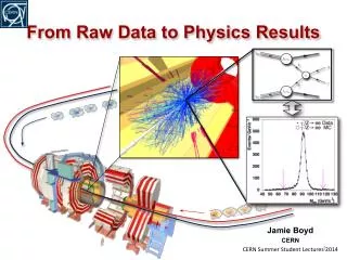
From Raw Data to Physics Results. Jamie Boyd CERN CERN Summer Student Lectures 2014. Outline. Summary Brief overview of the full lecture course A simple example Measuring the Z 0 cross-section Reconstruction & Simulation Track reconstruction Calorimeter recostruction

E N D
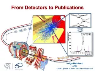
From Raw Data to Physics Results Jamie Boyd CERN CERN Summer Student Lectures 2014
Outline • Summary • Brief overview of the full lecture course • A simple example • Measuring the Z0 cross-section • Reconstruction & Simulation • Track reconstruction • Calorimeter recostruction • Physics object reconstruction • Simulation • Physics Analysis • Data Quality • Z’->ll • H->γγ • H->ZZ->4l • Computing infrastructure • The End! Todays Lecture • Disclaimer : Much of the content based on previous years lectures • Thanks to G. Dissertori
Data Analysis Chain • Have to collect data from many channels on many sub-detectors (millions) • Decide to read out everything or throw event away (Trigger) • Build the event (put info together) • Store the data • Analyze them • reconstruction, user analysis algorithms, data volume reduction • do the same with a simulation • correct data for detector effects • Compare data and theory This lecture course!!
DAQ chain (see lectures by W. Vandelli & B. Dahmes) Trigger data storage Main event Builder, High Level Trigger online reconstr. Detector Front-End . . . . . . . . . . . . Rate : MHz Rate : ~100 Hz Front-End Electronics 2 yes/no Detector 2 Upper Level Readout 2 Front-End Electronics 1 Detector 1 Upper Level Readout 1
Offline Analysis Chain offline reconstruction,calibration,alignment data storage further data storage . . . . Data size: PByte . . . . . . . . Data size: TByte User Analysis Program Data size: kByte
Data reduction/abstraction particle y detector element x Digitization/ Reconstruction ---> helix (R, d0, z0) Track finding + Track fit ---> hits (x1,y1,z1, t1) (x2,y2,z2, t2) ... Magnetic field B: reconstruct Event 1 px p = py pz Event 2 Track 1 Store theinfo for every event and every track <------- Analog signals Track 2 Track momentum
High Level Data Storage • Data are stored sequentially in files... Event 1 Event 2 Nch (charged tracks) : 3 Pcha (Momentum of each track): {{"-12.9305","12.2713","40.5615"}, {” 12.2469","-11.606","-38.7182"}, {"0.143435","-0.143435","-0.497444"}} pxpypz Qcha (Charge of each track): {-1,1,-1} Nch (charged tracks) : 2 Pcha(Momentum of each track): {{"-7.65698","42.9725","14.3404"}, {” 7.54101","-42.1729","-14.0108"}} pxpypz Qcha(Charge of each track): {-1,1} File A
Simulation process and detector simulation data storage . . . . . . . . • Simulation of many (billions) of events • simulate physics process • e.g. pp-> Zor pp-> H • plus the detector responseto the produced particles • understand detector response and analysis parameters (lost particles, resolution, efficiencies, backgrounds ) • and compare to real data • Note : simulations present from beginning to end of experiment, needed to make design choices Exactly the same steps as for the data
Our Task Reality We use experimentsto inquire about what“reality” (nature) does We intend to fill this gap • The goal is to understandin the most general; that’susually also the simplest. • - A. Eddington Theory
Theory... eg. the Standard Model has parameters coupling constants masses predicts: cross sections, branching ratios, lifetimes, ...
Experiment... • eg. • 1/30th of an event in the BaBar detector • get about 100 evts/sec • “Address” : • which detector element took the reading • “Value(s)” : • what the electronics wrote out
Making the connection Reality The imperfect measurement of a (set of) interactions in the detector Raw Data A unique happening:eg. Run 23458, event 1345which contains a Z → μ+μ- decay Reconstructed Events • Analysis : We “confront theory with experiment” by comparing • the measured quantity (observable) with the prediction. cross sections (probabilities for interactions), branching ratios (BR), ratios of BRs, specific lifetimes, ... Observables Theory A small number of general equations, with some parameters (poorly or not known at all)
Measuring Z0 cross-section at LHC • Z0 boson decays to lepton or quark pairs • We can reconstruct it in the e+e- or μ+μ- decay modes • Discovery and study of the Z0 boson was a critical part of understanding the electroweak force • Measuring the Z0 cross-section at the LHC important test of theory • Does the measurement agree with the theoretical prediction at LHC collision energy? • Now we use the Z0 as a tool for studying electron and muon reconstruction and deriving calibrations (have now recorded millions of Z decays) e+ q Z0 e- q Z0 cross-section is related to the probability that we will produce a Z0 at the LHC
Reconstructing Z0’s How do we know if it’s a Z0: Identify Z decays using the invariant mass of the 2 leptons M2 = (L1+L2)2 where Li = (Ei,pi) = 4-vector for lepton i Under assumption that lepton is massless compared to mass of Z0 => M2 = 2 E1 E2 (1-cosϑ12) where ϑ12= angle between the leptons So need to reconstruct the electron and muon energy and direction. Then can calculate the mass. • Select Z0 events with ‘analysis cuts’: • Events with 2 high momentum electrons or muons • Require the electrons or muons are of opposite charge • - With di-lepton mass close to the Z0 mass (e.g. 70<ml+l-<110 GeV) Very little background in the Z0 mass region
Slide taken from: “The achievements of the CERN proton – antiproton collider”, Luigi DiLella, 2004
Measuring the Z0 cross-section Theoretically: Cross-section calculated for: - Specific production mechanism (pp, pp, e+e-) - Centre-of-Mass of the collisions (7TeV at LHC) Experimentally: σ(pp->Z) = (NOBS – NBKG)/ Lε Where: NOBS = Number of observed events passing the selection NBKG = Estimate of the number of background events L = Luminosity of the data samples (amount of data) ε = Efficiency of the selection on Z0 events (how often would we select a true Z0 event with our selection?) e+/μ+ q Z0 e-/μ- q Can use simulated data to evaluate ε and NBKG
Measuring the Z0 cross-section σ(pp->Z) = (NOBS – NBKG)/ Lε Looks like simple counting experiment. But need to also calculate uncertainty on the cross-section – measurement without an uncertainty is useless. Two components to the uncertainty: Statistical: ~√NOBS Systematic: - How well do we know the background? - How well do we know the efficiency? - How well do we know the luminosity? Most of the work in the physics analysis is trying to understand the systematic uncertainties related to the above questions. Theory prediction Electron and Muon channel agree within uncertainties Measurement consistent with prediction within uncertainties Measurements of the Z cross-section were one of the first physics measurements from ATLAS and CMS.
Analysis flow in Z cross-section measurement Detector & Trigger Simulated data Reconstruct El and Mu candidates Reconstruction Reconstruction Select events with 2 oppositely charged El/Mu Calculate mass Select events with mass close to Z mass Physics Analysis Physics Analysis Compare theory and experiment
Analysis flow in Z cross-section measurement Detector & Trigger Simulated data Centrally produced by the collaboration Reconstruction Reconstruction Physics Analysis Physics Analysis Carried out by individuals or small analysis teams Compare theory and experiment
Summary • Path from Raw data to physics results contains many steps • Online path (Trigger and DAQ) • Offline path • Reconstruction • Physics Analysis • Use simulation in order to compare data with theoretical predictions • Above points illustrated with the example of the Z0 cross-section measurement at the LHC • More details on Monday
Reconstruction • Detector reconstruction • Tracking • finding path of charged particles through the detector • Calorimeter reconstruction • finding energy deposits in calorimeters from charged and neutral particles • Combined reconstruction • Electron/Photon identification • Muon identification • Jet finding • Calibrations and alignments applied at nearly every step
Important figures of merit for reconstructed objects • Efficiency • how often do we reconstruct the object – e.g. tracking efficiency Efficiency = (Number of Reconstructed Tracks) / (Number of True Tracks)
Important figures of merit for reconstructed objects • Efficiency • how often do we reconstruct the object – e.g. tracking efficiency • Resolution • how accurately do we reconstruct it – e.g. energy resolution Electron energy resolution from simulation Energy resolution = (Measured_Energy – True_Energy)/ True_Energy
Important figures of merit for reconstructed objects • Efficiency • how often do we reconstruct the object – e.g. tracking efficiency • Resolution • how accurately do we reconstruct a quantity – e.g. energy resolution • Fake rate • how often we reconstruct a different object as the object we are interested in – e.g. a jet faking a electron Fake rate = (Number of jets reconstructed as an electron) / (Number of jets)
Important figures of merit for reconstructed objects • Efficiency • how often do we reconstruct the object – e.g. tracking efficiency • Resolution • how accurately do we reconstruct a quantity – e.g. energy resolution • Fake rate • how often we reconstruct a different object as the object we are interested in – e.g. a jet faking a electron These quantities depend on the detector, but also on the reconstruction and calibrations and alignment!
Important figures of merit for reconstructed objects • Efficiency • how often do we reconstruct the object – e.g. tracking efficiency • Resolution • how accurately do we reconstruct a quantity – e.g. energy resolution • Fake rate • how often we reconstruct a different object as the object we are interested in – e.g. a jet faking a electron For physics analysis it is important to have high efficiency, good resolution, and low fake rates to be able to measure the efficiencies, resolutions and fake rates and their uncertainties (not easy)
Reconstruction Goals • High efficiency • Good resolution • Low fake rate • Robust against detector problems • Noise • Dead regions of the detector • Be able to run within the computing resources limitations • CPU time per event • Memory use