Download
1 / 31
310 likes | 644 Views
Spray and Wait: An Efficient Routing Scheme for Intermittently Connected Mobile Networks. Thrasyvoulos Spyropoulos, Konstantinos Psounis, Cauligi S. Raghavendra (All from the University of Southern California) SIGCOMM-2005, Philadelphia Presented by: Harshal Pandya

E N D
Spray and Wait: An Efficient Routing Scheme forIntermittently Connected Mobile Networks Thrasyvoulos Spyropoulos, Konstantinos Psounis, Cauligi S. Raghavendra (All from the University of Southern California) SIGCOMM-2005, Philadelphia Presented by: Harshal Pandya On 10/31/2006 for CS 577 - Advanced Computer Networks
Abstract • Intermittently Connected Mobile Networks (ICMN) are sparse wireless networks where most of the time there does not exist a complete path from the source to the destination. It can be viewed as a set of disconnected, time-varying clusters of nodes • These fall into the general category of Delay Tolerant Networks, where incurred delays can be very large and unpredictable. • Some networks that follow this paradigm are: • Wildlife tracking sensor networks • Military networks • Inter-planetary networks • In such networks conventional routing schemes such as DSR & AODV would fail ABSTRACT Introduction Related Work Spray & Wait Optimization Simulation Conclusion
An example of Intermittently Connected Mobile Networks (ICMN) • S is the source & D is the Destination • There is no direct path from S to D • In this case all the conventional protocols would fail • Thus, the authors introduce a new routing scheme, called Spray and Wait, that “sprays” a number of copies into the network, and then “waits” till one of these nodes meets the destination. 1 12 D 13 S 14 2 16 11 15 3 7 4 5 8 10
Basic Idea behind Spray & Wait • In such networks, the traditional protocols will fail to discover a complete path or will fail to converge, resulting in a deluge of topology update messages • However, this does not mean that packets can never be delivered in such networks • Over time, different links come up and down due to node mobility. If the sequence of connectivity graphs over a time interval are overlapped, then an end-to-end path might exist • This implies that a message could be sent over an existing link, get buffered at the next hop until the next link in the path comes up, and so on, until it reaches its destination • This approach imposes a new model for routing. Routing consists of a sequence of independent, local forwarding decisions, based on current connectivity information and predictions of future connectivity information • In other words, node mobility needs to be exploited in order to overcome the lack of end-to-end connectivity and deliver a message to its destination Abstract INTRODUCTION Related Work Spray & Wait Optimization Simulation Conclusion
A possible solution Abstract INTRODUCTION Related Work Spray & Wait Optimization Simulation Conclusion 1 12 D 13 S 14 2 16 11 15 3 7 4 5 8 10
Advantages of Spray & Wait • Under low load, Spray and Wait results in much fewer transmissions and comparable or smaller delays than flooding-based schemes • Under high load, it yields significantlybetter delays and fewer transmissions than flooding-based schemes • It is highly scalable, exhibiting good and predictable performance for a large range of network sizes, node densities and connectivity levels. As the size of the network and the number of nodes increase, the number of transmissions per node that Spray and Wait requires in order to achieve the same performance, decreases • It can be easily tuned online to achieve given QoS requirements, even in unknown networks • Using only a handful of copies per message, it can achieve comparable delays to an oracle-based optimal scheme that minimizes delay while using the lowest possible number of transmissions Abstract INTRODUCTION Related Work Spray & Wait Optimization Simulation Conclusion
Related Work • A large number of routing protocols for wireless ad-hoc networks have been proposed in the past. The performance of such protocols would be poor even if the network was only slightly disconnected • When the network is not dense enough (as in the ICMN case), even moderate node mobility would lead to frequent disconnections • In most cases trepairis expected to be larger than the path duration, this way reducing the expected throughput to almost zero according to the formula: • PD = average Path Duration • Another approach to deal with disconnections is to reinforce connectivity on demand, by bringing additional communication resources into the network when necessary (e.g. satellites, UAVs, etc.) Abstract Introduction RELATED WORK Spray & Wait Optimization Simulation Conclusion
Related Work • Similarly, one could force a number of specialized nodes (e.g. robots) to follow a given trajectory between disconnected parts of the network in order to bridge the gap • There, a number of algorithms with increasing knowledge about network characteristics like upcoming contacts, queue sizes, etc. is compared with an optimal centralized solution of the problem, formulated as a linear program • A number of mobile nodes performing independent random walks serve as DataMules that collect data from static sensors and deliver them to base stations • In a number of other works, all nodes are assumed to be mobile and algorithms to transfer messages from any node to any other node, are sought for • Epidemic Routing: • Here, each node maintains a list of all messages it carries, whose delivery is pending. Whenever it encounters another node, the two nodes exchange all messages that they don’t have in common. This way, all messages are eventually spread to all nodes, including their destination • But it creates a lot of contention for the limited buffer space and network capacity of typical wireless networks, resulting in many message drops and retransmissions Abstract Introduction RELATED WORK Spray & Wait Optimization Simulation Conclusion
Related Work • Randomized Flooding: • One simple approach to reduce the overhead of flooding and improve its performance is to only forward a copy with some probability p < 1 • History-based orUtility-based Routing: • Here, each node maintains a utility value for every other node in the network, based on a timer indicating the time elapsed since the two nodes last encountered each other. These utility values essentially carry indirect information about relative node locations, which get diffused through nodes’ mobility • Nodes forward message copies only to nodes with a higher utility by some pre-specified threshold value Uthfor the message’s destination. Such a scheme results in superior performance than flooding • But these schemes face a dilemma when choosing the utility threshold • Oracle-based algorithm: • This algorithm is aware of all future movements, and computes the optimal set of forwarding decisions (i.e. time and next hop), which delivers a message to its destination in the minimum amount of time. • This algorithm cannot be implemented practically, but is quite useful to compare against proposed practical schemes Abstract Introduction RELATED WORK Spray & Wait Optimization Simulation Conclusion
What should we expect from Spray & Wait ? • Perform significantly fewer transmissions than epidemic and other flooding-based routing schemes, under all conditions • Generate low contention, especially under high traffic loads • Achieve a delivery delay that is better than existing single and multi-copy schemes, and close to the optimal • Be highly scalable, that is, maintain the above performance behavior despite changes in network size or node density • Be simple and require as little knowledge about the network as possible, in order to facilitate implementation • Decouple the number of copies generated per message, and therefore the number of transmissions performed, from the network size • Thus it should be a tradeoff between single and multi-copy schemes. Abstract Introduction Related Work SPRAY & WAIT Optimization Simulation Conclusion
Definition • Definition 3.1 : Spray and Wait routing consists of the following two phases: • Spray phase:For every message originating at a source node, L message copies are initially spread – forwarded by the source and possibly other nodes receiving a copy – to L distinct “relays” • Wait phase:If the destination is not found in the spraying phase, each of the L nodes carrying a message copy performs direct transmission (i.e. will forward the message only to its destination) • This does not tell us how the Lcopies of a message are to be spread initially. So an improvement over Spray & Wait is Binary Spray & Wait Abstract Introduction Related Work SPRAY & WAIT Optimization Simulation Conclusion
Binary Spray & Wait • Binary Spray & Wait: • The source of a message initially starts with L copies; any node A that has n > 1 message copies, and encounters another node B with no copies, hands over to B, n/2 and keeps n/2 for itself; when it is left with only one copy, it switches to direct transmission • To prove that Binary Spray and Wait is optimal, when node movement is IID, the authors state and prove a theorem • Theorem 3.1: When all nodes move in an IID manner, Binary Spray and Wait routing is optimal, that is, has the minimum expected delay among all spray and wait routing algorithms • Proof: Let us call a node active when it has more than one copies of a message. Let us further define a spraying algorithm in terms of a function f : N → N as follows • When an active node with n copies encounters another node, it hands over to it f(n) copies, and keeps the remaining 1 − f(n) Abstract Introduction Related Work SPRAY & WAIT Optimization Simulation Conclusion
Binary Spray & Wait • Any spraying algorithm (i.e. any f) can be represented by the following binary tree with the source as its root: Assign the root a value of L; if the current node has a value n > 1 create a right child with a value of 1−f(n) and a left one with a value of f(n); continue until all leaf nodes have a value of 1 • A particular spraying corresponds then to a sequence of visiting all nodes of the tree. This sequence is random. On the average, all tree nodes at the same level are visited in parallel • Further, since only active nodes may hand over additional copies, the higher the number of active nodes when icopies are spread, the smaller the residual expected delay • Since the total number of tree nodes is fixed (21+log L − 1) for any spraying function f, it is easy to see that the tree structure that has the maximum number of nodes at every level, also has the maximum number of active nodes at every step. • This tree is the balanced tree, and corresponds to the Binary Spray and Wait routing scheme. As Lgrows larger, the sophistication of the spraying heuristic has an increasing impact on the delivery delay of the spray and wait scheme. Abstract Introduction Related Work SPRAY & WAIT Optimization Simulation Conclusion
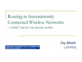
Binary Spray & Wait • Figure compares the expected delay of Binary Spray & Wait and Source Spray & Wait as a function of the number of copies Lused, in a 100×100 network with 100 nodes • This figure also shows the delay of the Optimal scheme. Abstract Introduction Related Work SPRAY & WAIT Optimization Simulation Conclusion As the number of copies of the message increase, the Spray & Wait Mechanism slowly moves towards optimality. Binary Spray & Wait is better than Source Spray & Wait
Optimizing Spray & Wait • In many situations the network designer or the application itself might impose certain performance requirements on the protocols (e.g. maximum delay, maximum energy consumption, minimum throughput, etc.). • Spray and Wait can be tuned to achieve the desired performance. • To do so the authors summarize a few results regarding the expected delay of the Direct Transmission and Optimal schemes • Lemma 4.1: Let M nodes with transmission range K perform independent random walks on a torus. • The expected delay of Direct Transmission is exponentially distributed with average Abstract Introduction Related Work Spray & Wait OPTIMIZATION Simulation Conclusion
Optimizing Spray & Wait • The expected delay of the Optimal algorithm is: • Lemma 4.2: The expected delay of Spray and Wait, when L message copies are used, is upper-bounded by: This bound is tight when L << M Abstract Introduction Related Work Spray & Wait OPTIMIZATION Simulation Conclusion
Choosing L to Achieve a RequiredExpected Delay • Assume that there is a specific delivery delay constraint to be met. This delay constraint is expressed as a factor a times the optimal delay EDopt(a > 1) • Lemma 4.3: The minimum number of copies Lmin needed for Spray and Wait to achieve an expected delay at most a*EDopt, is independent of the size of the network N and transmission range K, and only depends on a and the number of nodes M • Thus we get the following equation from the previous upper bounded equation of EDsw Note : EDsw= a*EDopt and approximate the harmonic number HM−L with its Taylor Series terms up to second order, and solve the resulting third degree polynomial Abstract Introduction Related Work Spray & Wait OPTIMIZATION Simulation Conclusion
Comparing Various L • L found through the approximation is quite accurate when the delay constraint is not too stringent. Abstract Introduction Related Work Spray & Wait OPTIMIZATION Simulation Conclusion
Estimating Lwhen Network Parametersare Unknown • In many casesboth Mand N, might be unknown • But for determining L, at least M is required • Hence we have to somehow estimate M to find out L • A straightforward way to estimate Mwould be to count unique IDs of nodes encountered already. This method requires a large database of node IDs to be maintained in large networks, and a lookup operation to be performed every time any node is encountered • A better method: We define T1 as the time until a node encounters anyother node. T1 is exponentially distributed with average T1 = EDdt/(M − 1) • We similarly define T2 as the time until two different nodes are encountered, then the expected value of T2 equals EDdt (1/(M-1) + 1/(M-2)) • Canceling EDdtfrom these two equations we get the following estimate for M: Abstract Introduction Related Work Spray & Wait OPTIMIZATION Simulation Conclusion
A better estimate of T1 & T2 • When a random walk i meets another random walk j, i and j become coupled • In other words, the next inter meeting time of i and j is not anymore exponentially distributed with average EDdt • In order to overcome this problem, each node keeps a record of all nodes with which it is coupled • Every time a new node is encountered, it is stamped as coupled for an amount of time equal to the mixing or relaxation time for that graph • Then, when node Imeasures the next sample inter meeting time, it ignores all nodes that it’s coupled with at the moment, denoted as ck, and scales the collected sample T1,kby (M−ck)/(M−1) • A similar procedure is followed for T2. Putting it altogether, after n samples have been collected: Abstract Introduction Related Work Spray & Wait OPTIMIZATION Simulation Conclusion
Comparing the online estimators of M • This method is more than two times faster than ID counting Abstract Introduction Related Work Spray & Wait OPTIMIZATION Simulation Conclusion Estimated value of M quickly converges with the actual value
Scalability of Spray and Wait • As the number of nodes in the network increases, the percentage of nodes (Lmin/M) that need to become relays in Spray and Wait to achieve the same performance relative to the optimal, actually decreases • Also, the performance of Spray & Wait improves faster than optimal scheme !!! This can be proved using Lemma 4.4 Abstract Introduction Related Work Spray & Wait OPTIMIZATION Simulation Conclusion
Spray and Wait actually decreases the transmissions per node as the number of nodes Mincreases • Lemma 4.4: Let L/M be constant and let L << M. Let further Lmin(M) denote the minimum number of copies needed by Spray and Wait to achieve an expected delay that is at most a*EDopt, for some a. Then Lmin(M)/M is a decreasing function of M. Abstract Introduction Related Work Spray & Wait OPTIMIZATION Simulation Conclusion
Scenario A : Effect of Traffic Load • Assumptions: • 100 nodes move according to the random waypoint model in a 500 × 500 grid with reflective barriers. • The transmission range Kof each node is equal to 10 • Each node is generating a new message for a randomly selected destination with an inter-arrival time distribution uniform in [1, Tmax] until time 10000 • Tmaxis variedfrom 10000 to 2000 creating average traffic loads from 200 (low traffic) to 1000 (high traffic). Abstract Introduction Related Work Spray & Wait Optimization SIMULATION Conclusion Spray & Wait is significantly better than other schemes
Scenario B : Effect of Connectivity • The size of the network is 200×200 and Tmaxis fixed to 4000 (medium traffic load). The number of nodes Mand transmission range K, are variedto evaluate the performance of all protocols in networks with a large range of connectivity characteristics, ranging from very sparse, highly disconnected networks, to almostconnected networks. Abstract Introduction Related Work Spray & Wait Optimization SIMULATION Conclusion As the transmission range increases more & more nodes fall within the range of each other & the percentage of nodes in the max cluster increases
Scenario B: Number of transmissions for various transmission ranges for 100 & 200 nodes Abstract Introduction Related Work Spray & Wait Optimization SIMULATION Conclusion For both networks, the number of transmissions for spray and wait are very less in number as compared to other schemes & are also more or less independent from the transmission range K
Scenario B: Delivery delay for various transmission ranges for 100 & 200 nodes The delivery delay of Spray and Wait is significantly better than that of other schemes & depends on the transmission range. As the transmission range increases the delay decreases.
Conclusion • Spray and Wait effectively manages to overcome the shortcomings of epidemic routing and other flooding-based schemes, and avoids the performance dilemma inherent in utility-based schemes • Spray and Wait, despite its simplicity, outperforms all existing schemes with respect to number of transmissions and delivery delays, achieves comparable delays to an optimal scheme, and is very scalable as the size of the network or connectivity level increase Abstract Introduction Related Work Spray & Wait Optimization Simulation CONCLUSION
Some issues not discussed • Power consumed • Security • Constrained Mobility of Nodes
Acknowledgements • The slide design has been adopted from the presentation by Mike Putnam (Because I liked it a lot) • Some figures have been adopted from the presentation by the authors • All other figures have been taken from the actual paper
Thank you Questions ?