Download
1 / 16
160 likes | 492 Views
Mapping genes with LOD score method. LOD score method. Aim: Determine , the recombinant fraction (fraction of gametes that are recombinant), using data from relatively small families. Reminder: vary from 0 (2 genes completely linked) to 0.5 (2 genes are unlinked).

E N D
LOD score method • Aim: Determine , the recombinant fraction (fraction of gametes that are recombinant), using data from relatively small families. • Reminder: vary from 0 (2 genes completely linked) to 0.5 (2 genes are unlinked).
LOD score method (cont.) There are 4 basic steps in the process: • Determine the expected frequencies of F2 phenotypes for every value of from 0.01 to 0.5 • Determine the “likelihood” (L) that the family data observed resulted from the given value: the maximum likelihood is the best estimate of for given data. • Determine the Odds Ratio and logarithm of the odds ratio (lod score) by comparing the Likelihood for each value of to the Likelihood for unlinked genes (=0.5) • Add lod scores from different families to achieve an acceptably high lod score so a specific most likely can be assigned.
a b A B P: x a b A B A B F1: A B x a b a b A_ B_ A_ bb F2: aa B_ aa bb LOD score method (cont.) Lets see how it works on two genes showing complete dominance:
LOD score method (cont.) Step 1: Calculate the expected frequency of offspring for values of fro 0.01 to 0.5 Example: Lets calculate expected offspring number for =0.2: • P(Ab)=P(aB)=0.1 ; P(AB)=P(ab)=0.4 2. • F2 phenotype cell sums expected freq
LOD score method (cont.) Step 2: Estimate the observed family data in light of the expected distribution of offspring for each R value. This is done by determining likelihood (L) of the observed family for each value of R. The likelyhood is simply the probability of the observed family, as determined by the multinomial theorem (see http://mathworld.wolfram.com/MultinomialDistribution.html) Lets define our terms for the observed family: • a = number of A_ B_ offspring • b = number of A_ bb offspring • c = number of aa B_ offspring • d = number of aa bb offspring • n = total offspring (a+b+c+d)
LOD score method (cont.) …and terms for the expected family proportions (obtained fro Step1 above): • p = expected proportion of A_ B_ offspring • q = expected proportion of A_ bb offspring • r = expected proportion of aa B_ offspring • s = expected proportion of aa bb offspring Then Likelihood will be calculated by the next formula:
LOD score method (cont.) Example: A family as in previous example has 5 children: 2 of A_ B_ phenotype, 1 with aa B_ and 2 with aa bb. What is the likelihood of this family, given =0.2? L=(5!/2!0!1!2!)(0.66)2(.09)0 (.09)1 (.16)2=0.0301
LOD score method (cont.) Steps 3 and 4: Combining data from several families. We want to be able to compare (and add) data from several different families, to get a good estimate of R. To do this, the L values must be standardized by calculating Odds Ratio (OR), which is the ratio of the L for each value divided by the L for =0.5 . Then, the logarithm of Odds Ratio is taken; this is the lod score (Z). Lod scores from different families can be added (this is equivalent to multiplying the Odds Ratios, as in the AND rule for two events – family 1 and family 2 – both occurring). A total lod score for some value of 3.0 is considered proof of linkage between two genes, which is not exactly right as will be explained futher…
Exclusion Mapping In linkage analysis the main goal is localizing disease genes relative to well-characterized marker loci (lod score > 3). However with any given marker, the probability of finding a positive test result is quite low as human genome is quite large and most randomly selected markers are not linked. However, negative results are also results and may be used for elimination of various chromosomal regions from consideration…
Exclusion Mapping (cont.) It’s important to remember that the likelihood ratio test is a test of hypothesis of no linkage, such that in the absence of a significant test result, you fail to reject H0, meaning that there is no significant evidence for linkage. However, this does not mean that you accept H0 and have proved by the failure to achieve a significant test result that there is no linkage. It’s quite another thing to prove the absence of linkage – a problem that can be statistically very complicated…
Exclusion Mapping (cont.) Morton has proposed (1955) that the test of linkage be treated as a sequential likelihood ratio test (LRT) of a simple hypothesis, = 1. He proposed that the new families continue to be sampled until either the criterion Z(1)>3 is fulfilled, in which case the hypothesis of no linkage is rejected, or until Z(1)<-2, in which case you would reject the hypothesis of linkage. As long as -2<Z(1)<3, no conclusion may be made.
Exclusion Mapping (cont.) Chotai (1984) extended this concept to the general case such that the positive test is considered significant whenever Zmax>3; and the negative test is considered significant on { | Z () < -2}, and the disease gene may be excluded from this part of genome. The same criteria may be applied for both two-point and multipoint scores…
Model Errors and Exclusion Mapping It has bee shown that using incorrect model for the disease doesn’t in general lead to an increased false-positive rate (Clerget-Darpoux et al., 1986), as maximizing the lod score over models does (Weeks et al. 1990a). In other words, you are not more likely to obtain lod scores of 3 in the absence of linkage under the wrong model than using the correct one… If there is linkage, however, there is lower power to detect it when the model parameters are incorrectly specified…
Model Errors and Exclusion Mapping (cont.) Contrary to the lack of false-positives, the false-negative rate may be astronomical when an analysis is performed under incorrect model. It’s quite easy to design an example where disease gene will be mistakenly “excluded” from it’s region by Z()<-2 criterion: If there is a linkage in only 20% of families, then summing the lod scores across the families can easily lead us to spurious exclusions.
Model Errors and Exclusion Mapping (cont.) For this reason, doing a linkage analysis with a complex disease, for which the model is not accurately known, it’s not wise to use exclusion analysis because the exclusion results obtained apply only to that specific model. You can only say that this region may be excluded only if the analysis model is correct…