Download
1 / 26
260 likes | 358 Views
Discover how genes contributing to mouse traits are mapped using crosses of inbred strains. Learn about loci, markers, genotype calling, and Mendel's laws for one and two loci.

E N D
How many genes? Mapping mouse traits Lecture 1, Statistics 246 January 20, 2004
To review basic Mendelian genetics, the basics of recombination, and go on to see how genes contributing to qualitative and quantitative traits are mapped using data from crosses of inbred strains of mice. Aim of today’s and Thursday’s lecture
2.1 Loci and markers We need to know the following notions from Meldelian genetics: autosomes, sex chromosomes, genotypes, phenotypes, loci, alleles, homozygous, heterozygous, dominant, recessive, (fully) inbred, markers. 2.1 Genetic background
Our markers are Microsatellites ..AGTCCACACACACACACATGT.. ..AGTCCACACACACACACATGT.. A PCR and electrophoresis ..AGTCCACACACACACACATGT.. ..AGTCCACACACACACACACACACATGT.. H ..AGTCCACACACACACACACACACATGT.. ..AGTCCACACACACACACACACACATGT.. B Desirable: to call the genotypes (A, H, or B) automatically Problems: stutters and noise, variability of the patterns, etc.
Similarity Sorting unsorted sorted correlation matrix This is a useful technique to enhance presentation of gel traces and assist manual examination.
Genotype Calling • This is a statistical pattern recognition problem: • Fit mixture models • Discriminant analysis A H B
Our main players are the C57BL/6 (BL for black, abbreviated B6), a robust strain that has been around about 90 years, and the NOD (non-obese diabetic) mouse strain, a delicate diabetes-prone strain discovered in 1990. Coat colours: agouti is standard, B6 is black, NOD is albino (i.e. white). 2.2 Inbred strains and their crosses
Normal (wild-type) mouse coat: color = agouti a grizzled color of fur resulting from the barring of each hair in several alternate dark and light bands
Four main loci : A, B, C and D Locus A – agouti Locus B – black Locus C (known as Tyr) – albinism Locus D – dilution gene Coat color loci in mice
Ay, Lethal dominant yellow Avy, Viable yellow Aw, White-bellied Agouti A, Agouti or Wild type At, Black and Tan Am, mottled agouti a, Non-agouti ae., Extreme non-agouti A and a are a dominant/recessive allele pair Alleles at the Agouti (A) locus
C, full color gene cch, chincilla ch, himalayan c, albino gene C and c are a dominant/recessive pair of alleles Alleles at the Albino (C) Locus
If the mouse is aaCx it is not agouti and not albino (in our case a black mouse) If the mouse is AxCx it is agouti and not albino If the mouse is xxcc it is albino no matter what the alleles at the agouti locus are because they are irrelevant Alleles at A and C interact (called epistasis in genetics)
We will denote the NOD mice by A, and the B6 mice by B. This same notation will denote the two homozygotes at a polymorphic marker. Two main crosses interest us, following the first filial generation or F1 , which we denote by AB H. Here H denotes heterozygote, which is the case for our F1s. The backcross BC is arrived at via HB BC, or a variant, while the F2intercross is given by HH F2. Crosses
An F2 inter cross was performed starting with C57BL/6 and NOD parental lines. We have 133 female mice at the F2 generation, just females for the reason that males fight, and this influences other (quantitative blood) phenotypes of interest They were genotyped at 153 microsatellite markers spanning all 19 autosomes and the X chromosome. We also have coat color and a few white blood cell phenotypes. 2.3 Data
A small portion of the data (beginning) #individuals #loci #traits marker next column = data from mouse1 D10M106 = a marker on chr 10 defined by MIT Incompleteness code: C = B or H, D = A or H, - = missing
A small portion of the raw data (end) Coat color code WBC traits
Using the LOD_error statistic. Based on close recombn events which indicate possible presence of genotyping error (see later) Error Detection calc.genoprob, calc.errorlod, plot.errorlod
We can (and should) check Mendel with data from our 133 offspring at each of our 153 loci. For example, at D7Mit126, we have 24 A, 29 B and 67 H genotypes, adding to 120, indicating 12 incomplete or missing genotypes. What do we expect according to Mendel? How would we test whether the data agree with our expectations? 2.4 Mendel’s laws for one locus
Mendel inferred from his data on peas the independent segregation of different factors. Here we check that this holds for our two coat color loci, but not generally. We then go on to understand the more general situation. 2.5 Mendel’s law for 2 loci
Mating & Coat color outcomes in this cross C57/BL6 males Black (aaBBCC) NOD females Albinos (AABBcc) Parental lines All Agouti aABBCc F1 Agouti : 9 Black : 3 Albino 4 F2 We need to check these last proportions following Mendel’s reasoning.
Punnett square depicting F1 parental allele combinations passed on to F2 offspring
It’s not always like that 2-locus genotypes at D12Mit51 and D12Mit132. If we pool A and H, we do not get 9:3:3:1.