Ch 7 Capital asset pricing model and arbitrage pricing model

1. Ch 7 Capital asset pricing model and arbitrage pricing model

2. Capital Asset Pricing Model (CAPM) Equilibrium model that underlies all modern financial theory Derived using principles of diversification with simplified assumptions Markowitz, Sharpe, Lintner and Mossin are researchers credited with its development

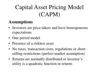
3. Assumptions Individual investors are price takers Single-period investment horizon Investments are limited to traded financial assets No taxes, and transaction costs

4. Assumptions (cont.) Information is costless and available to all investors Investors are rational mean-variance optimizers Homogeneous expectations

5. Resulting Equilibrium Conditions All investors will hold the same portfolio for risky assets – market portfolio Market portfolio contains all securities and the proportion of each security is its market value as a percentage of total market value

6. Resulting Equilibrium Conditions (cont.) Risk premium on the market depends on the average risk aversion of all market participants Risk premium on an individual security is a function of its covariance with the market

7. Figure 7-1 The Efficient Frontier and the Capital Market Line

8. Slope and Market Risk Premium M = Market portfolio rf = Risk free rate E(rM) - rf = Market risk premium E(rM) - rf = Market price of risk s M

9. Expected Return and Risk on Individual Securities The risk premium on individual securities is a function of the individual security’s contribution to the risk of the market portfolio Individual security’s risk premium is a function of the covariance of returns with the assets that make up the market portfolio

10. Figure 7-2 The Security Market Line and Positive Alpha Stock

11. SML Relationships b = [COV(ri,rm)] / sm2 Slope SML = E(rm) - rf = market risk premium SML = rf + b[E(rm) - rf]

12. Sample Calculations for SML E(rm) - rf = .08 rf = .03 bx = 1.25 E(rx) = .03 + 1.25(.08) = .13 or 13% by = .6 e(ry) = .03 + .6(.08) = .078 or 7.8%

13. Graph of Sample Calculations E(r) SML Rx=13% .08 Rm=11% Ry=7.8% 3% ß .6 1.0 1.25 ß ß ß y m x

14. Estimating the Index Model Using historical data on T-bills, S&P 500 and individual securities Regress risk premiums for individual stocks against the risk premiums for the S&P 500 Slope is the beta for the individual stock

15. Table 7-1 Monthly Return Statistics for T-bills, S&P 500 and General Motors

16. Figure 7-3 Cumulative Returns for T-bills, S&P 500 and GM Stock

17. Figure 7-4 Characteristic Line for GM

18. Table 7-2 Security Characteristic Line for GM: Summary Output

19. Multifactor Models Limitations for CAPM Market Portfolio is not directly observable Research shows that other factors affect returns

20. Fama French Research Returns are related to factors other than market returns Size Book value relative to market value Three factor model better describes returns

21. Table 7-4 Regression Statistics for the Single-index and FF Three-factor Model

22. Arbitrage Pricing Theory Arbitrage - arises if an investor can construct a zero beta investment portfolio with a return greater than the risk-free rate If two portfolios are mispriced, the investor could buy the low-priced portfolio and sell the high-priced portfolio In efficient markets, profitable arbitrage opportunities will quickly disappear

23. Figure 7-5 Security Line Characteristics

24. APT and CAPM Compared APT applies to well diversified portfolios and not necessarily to individual stocks With APT it is possible for some individual stocks to be mispriced - not lie on the SML APT is more general in that it gets to an expected return and beta relationship without the assumption of the market portfolio APT can be extended to multifactor models

25. Exercise241 1. Stocks A, B, C and D have betas of 1.5, 0.4, 0.9 and 1.7 respectively. What is the beta of an equally weighted portfolio of A, B and C? A) .25 B) .93 C) 1.00 D) 1.13 2. The market portfolio has a beta of __________. A) -1.0 B) 0 C) 0.5 D) 1.0 3. According to the capital asset pricing model, a well-diversified portfolio's rate of return is a function of __________. A) market risk B) unsystematic risk C) unique risk D) reinvestment risk

26. Exercise 42 1. According to the capital asset pricing model, fairly priced securities have __________. A) negative betas B) positive alphas C) positive betas D) zero alphas 2. Consider the single factor APT. Portfolio A has a beta of 1.3 and an expected return of 21%. Portfolio B has a beta of 0.7 and an expected return of 17%. The risk-free rate of return is 8%. If you wanted to take advantage of an arbitrage opportunity, you should take a short position in portfolio __________ and a long position in portfolio __________. A) A, A B) A, B C) B, A D) B, B

27. Exercise22 1. Security X has an expected rate of return of 13% and a beta of 1.15. The risk-free rate is 5% and the market expected rate of return is 15%. According to the capital asset pricing model, security X is __________. A) fairly priced B) overpriced C) underpriced D) None of the above 2. If the simple CAPM is valid, which of the situations below are possible? Consider each situation independently. A) Situation A B) Situation B C) Situation C D) Situation D