S udden Stratospheric Warming Effects
190 likes | 409 Views
S udden Stratospheric Warming Effects. M . V . Klimenko , V . V . Klimenko , F . S . Bessarab , Yu . N . Koren’kov. WD Pushkov IZMIRAN, RAS, Kaliningrad, Russia, maksim . klimenko @ mail . ru.

S udden Stratospheric Warming Effects
E N D
Presentation Transcript
Sudden Stratospheric Warming Effects M.V. Klimenko, V.V. Klimenko, F.S. Bessarab, Yu.N. Koren’kov WD Pushkov IZMIRAN, RAS, Kaliningrad, Russia, maksim.klimenko@mail.ru
Sudden Stratospheric Warming is the example of the links between low- and middle-atmosphere and ionosphere • SSW is a dramatic, large scale meteorological process in the winter middle atmosphere which involves profound changes of temperature and circulation. SSW can last for several days or weeks. • A stratospheric warming is identified as major if at height of 30 km (10 mbar) or below, the zonal mean temperature increases poleward from ~60o latitude and an associated circulation reversal (breakdown of the polar vortex) are observed. • Minor warmings may reach comparable intensities (i.e., high temperatures), but do not lead to a breakdown of the circulation as is defined above.
Thermosphere Ionosphere Mesosphere Electrodynamics General Circulation Model (TIMEGCM) (30 – 600 км) Liu et al., 2002, 2005, 2010; Yamashita et al., 2010 Recent Model results Whole Atmospheric Model (WAM) (0 – 600 км ) Fuller-Rowell et al., 2011, 2010. Observed data Goncharenko et al, GRL 2010 Chau et al, JGR 2010 Model simulations
Pancheva and Mukhtarov., 2011 Day Number (start 1 October 2007) Day Number (start 1 October 2008)
Model GSM TIP Brief Description Thermospheric parameters: Tn, O2, N2, O, NO, N(4S),N(2D) densities; vector of velocities; (from 80 km to 500 km) Ionospheric parameters: O+, H+, Mol+ densities; Ti and Te; Vectors of ion velocities (from 80 km to 15 Earth radii) Electric field: The model is added by the new block of electric field calculation Klimenko et al., 2006, 2007. Global Self-consistent Model of the Thermosphere, IonosphereandProtonosphere(GSM TIP) was developed in West Department of IZMIRAN. The model GSM TIP was described in details inNamgaladze et al., 1988.
SSW-2009 January, 23 max Tn effect January, 27 max dynamical effect • Westward winds slowed down and reversed direction. Major SSW event. • Large and long lasting temperature increase. • Low solar activity and quiet geomagnetic conditions. • 11 days coverage with ISR measurements of the drifts and densities, and mesospheric dynamics.
First SSW scenario for 2009 COMMA-LIM model (Fröhlich et al., 2003). • Observation data • Incoherent scatter radar (ISR) electron density and temperature measurements from the Irkutsk, • as well as ionosonde data of • Yakutsk (62.2° N, 162.6° E) • Irkutsk (52.2° N, 104.0° E), • Kaliningrad (54.7°N, 20.6° E), • Jicamarca (12.0° S, 76.9° W) , • and St. Johns (STJ) (23.2° S, 45.9° W) Quasi-stationary PW with zonal wave number s = 1. The neutral temperature disturbances at lower boundary of GSM TIP model (80 км ).
Ti disturbances over Millstone Hill (Goncharenko and Zhang, 2008) Heating due to wave energy dissipation foF2 before SSW-event foF2 (Jan 27 – Jan 15)
SSW peak SSW min Tn in stratosphere 60-90N
Summary (1) • Using the presented approach allows to reproduce the observed perturbations of the neutral temperature in MLT region above Irkutsk and global negative ionospheric disturbances during 2008 and 2009 SSW events • Model calculations allowed to explain the observed global negative ionospheric disturbances during SSW events • Morning SSW positive effects in the electron density at low latitudes which have recently been discussed by Goncharenko et al. (2010), Chau et al. (2011), Fejer et al. (2011) are absent in our simulation results. • A more realistic description of neutral atmosphere parameters at altitudes of the mesopause region (lower boundary of the GSM TIP model) has to be used in order to reproduce the observed positive ionospheric disturbances at low latitudes during stratospheric warming events.
Another Scenario For 2009 SSW GSM TIP GlobalSelf-consistentModeloftheThermosphere, IonosphereandProtonosphere Tn, O2, N2, O, NO, N(4S),N(2D) densities; vectors of velocities (from 80 km to 500 km) O+, H+, Mol+ densities; Ti and Te; ion velocities (from 80 km to 15 Earth radii) Electric field SOCOL SOlar-Climate-Ozone Links model horizontal resolution: 3.75° vertical resolution: 39 levels to 0.01 hPa Winds and temperature, 41 chemical species TIME-GCM model Thermospheic output at 80 km Thermospheic output at 80 km ECMWFdata for SSW 2009 event Output at 30 km
Tn (Jan,21 – Jan, 15) on 60N foF2 (Jan,21 – Jan, 15) on 60N cooling of the north polar cap
ECMWF + TIME-GCM +GSM TIP GPS TEC IGS GPS TEC
Summary (2) • Mesospheric effects of SSW, as well as thermospheric and ionospheric effects simulated with GSM TIP, obtained in the second scenario are smaller than that in the first scenario. • The choice of a method for calculating the mean (background) values is important for interpreting the observed data. • Although a new scenario of SSW-2009 event qualitatively reproduces an increase in foF2 in a near-equatorial area, but observed magnitudes are much higher. • Is it possible to reproduce so big ionospheric disturbances at low latitudes using GSM TIP model?
Newest simulation obtained using GSM TIP model with taken into account observed E × B vertical plasma drift (zonal electric field) over the Jicamarca, Peru during SSW 2009 event Jicamarca, Peru 11.9°S, 76.0°W; -0.6°, 353.9° Porto Alegre, Brazil 30.1°S, 51.1°W; -19.2°, 17.1° Evonal on 15 January 2009 Ezonal on 25 January 2009 Millstone Hill, MA, USA 42.6°N, 71.5°W; 54.1°, 357.0° delta Evonal on 25 January 2009 Qaanaaq, Greenland 77.5°N, 69.1°W: 88.9°, 6.7°
TEC and it disturbances obtained using GSM TIP model with observed E × B vertical drift and GPS TEC data GSM TIP on 15 January 2009 GSM TIP on 25 January 2009 delta GSM TIP on 25 January 2009 GPS TEC on 15 January 2009 GPS TEC on 25 January 2009 delta GPS TEC on 25 January 2009
Modulation of GW by PW Hoffmann, Jacobi (2010) MetO temperature data (red line), SABER (green lines) and the modulation of GW potential energy (blue lines). dTEC (thick black line) indicate the possible ionospheric response to the waves coming from below Acknowledgments.The authors express their sincere thanks to Hanli Liu, EugenRozanov, Larisa Goncharenko, Marina Chernigovskaya, for the fruitful cooperation, providing the data and making the experimental data available. These investigations were supported by RFBR Grant No. 12-05-31217 and RAS Program 22.