Machine Learning I - Outline
Machine Learning I - Outline. Introduction to ML Definitions of ML ML as a multidisciplinary field A framework for learning Inductive Learning - Version Space Search - Decision Tree Learning. Introduction to ML.

Machine Learning I - Outline
E N D
Presentation Transcript
Machine Learning I - Outline • Introduction to ML • Definitions of ML • ML as a multidisciplinary field • A framework for learning • Inductive Learning - Version Space Search - Decision Tree Learning
Introduction to ML • The ability to learn is one of the most important components of intelligent behaviour • System good in doing a specific job • performs costly computations to solve the problem • does not remember solutions • every time it solves the problem it performs the same sequence of computations again • A successful understanding of how to make computers learn would open up many new uses of computers
Application Areas of ML • ML algorithms for: • computers learning from medical records which treatments are best for new diseases • speech recognition - recognition of spoken words • data mining - discovering of valuable knowledge from large databases of loan applications, financial transactions, medical records, etc. • prediction and diagnostics - prediction of recovery rates of pneumonia patients, detection of fraudulent use of credit cards • driving an autonomous vehicle - computer controlled vehicles ...
Machine Learning: Definitions • T. Mitchell (1997): A computer program learns if it improves its performance at some task through experience • T. Mitchell (a formal definition, 1997): A computer program is said to learn from experience E with respect to some class of tasks T and performance measure P, if its performance at tasks in T as measured by P, improves with experience E. • Definition of learning by H. Simon (1983): Any change in a system that allows it to perform better the second time on repetition of the same task or on task drawn from the same population.
Issues involved in the learning programs • Learning involves changes in the learner • Learning involves generalisation from experience • Performance should improve not only on the repetition of the same task but also on similar tasks in the domain • Learner is given a limited experience to acquire knowledge that will generalise correctly to unseen instances of the domain. This is the problem of induction • Learning algorithms must generalise heuristically – must select the important aspects of their experience • Learning algorithms must prevent and detect possibilities that changes in the system may actually degrade its performance
ML as Multidisciplinary Field Key ideas from the fields that impact ML: • AI - learning symbolic representations of concepts, using prior knowledge together with training data to guide learning • Bayesian methods - estimating values of unobserved variables • Computational complexity theory - theoretical bounds on complexity of different learning tasks • Control theory - procedures that learn to control processes and to predict the next state of the controlled process • Information theory - measures of entropy and information content, minimum description length approaches, optimal codes • Statistics - confidence intervals and statistical tests • Philosophy - Occam’s razor, suggesting that the simplest hypothesis is the best • Psychology and neurobiology - motivation for artificial neural networks
A Framework for Learning • A well-defined learning problem is identified by • class of tasks, • measure of performance to be improved, and • the source of experience. • Example 1: A checkers learning problem • Task: playing checkers • Performance measure: percent of games won against opponents • Training experience: playing practice games against itself
A Framework for Learning • Example 2: A handwriting recognition learning problem • Task: recognising and classifying handwritten words within images • Performance measure: percent of words correctly classified • Training experience: database of classified handwritten words • ML algorithms vary in their goals, in the representation of learned knowledge, in the available training data, and in the learning strategies • all learn by searching through a space of possible concepts to find an acceptable generalisation
Inductive Concept Learning: Definitions • What is induction? • Induction is reasoning from properties of individuals to properties of sets of individuals • What is a concept? • U - universal set of objects (observations) • a concept C is a subset of objects in U, CU • Examples: • C is a set of all black birds (if U is a set of all birds) • C is a set of mammalian (if U is a set of all animals) • Each concept can be thought of as a boolean-valued function defined over the set U
Inductive Concept Learning: Definitions • What is concept learning? • To learn a concept C means to be able to recognize which objects in U belong to C • What is inductive concept learning? • Given a sample of positive and negative training examples of the concept C • Find a procedure (a predictor, a classifier) able to tell, for each xU, whether xC
Concept Learning and the General-To-Specific Ordering • Concept learning as a problem of searching through a space of potential hypotheses for the hypothesis that best fits the training data • In many cases the search can be efficiently organised by taking advantage of a naturally occurring structure over the hypothesis space - a general-to-specific ordering of hypothesis • Version spaces and the Candidate-elimination algorithm
Describing objects and concepts • Formal description languages: • example space LE - language describing instances • hypothesis space LH - language describing concepts • Terminology: • hypothesis H - a concept description • example e=(ObjectDescription, ClassLabel) • positive example e+ - description of a positive instance of C • negative example e- - description of a non-instance • example set E: E = E+E- for learning a simple concept C • coverage: H covers e, if e satisfies (fulfils, matches) the conditions stated in H
Prototypical Concept Learning Task • Given: • Instances X: Possible days, each described by the attributes Sky, AirTemp, Humidity, Wind, Water, Forecast • Target function c: EnjoySport: X{0,1} • Hypotheses H: Conjunctions of literals. E.g. ?,Cold,High,?,?,?. • Training examples E: Positive and negative examples of the target function x1,c(x1),…, xm,c(xm). • Determine: A hypothesis h in H such that h(x)=c(x) for all x in E.
Representing Hypothesis • Many possible representations • Here, h is conjunction of constraints on attributes • Each constraint can be • a specific value (e.g. Water=Warm) • don’t care (e.g. Water=?) • no value allowed (e.g. Water=) • Example: SkyAirTempHumidWindWaterForecast Sunny ? ? Strong ? Same
Training Examples for Enjoy Sport Sky Temp Humidity Wind Water Forecast EnjoySport Sunny Warm Normal Strong Warm Same YES Sunny Warm High Strong Warm Same YES Rainy Cold High Strong Warm Change NO Sunny Warm High Strong Cool Change YES What is the general concept?
is more_general_than_or_equal_to relation • Definition of more_general_than_or_equal_to relation: Let hj and hk be boolean-valued functions defined over X. Then hjis more_general_than_or_equal_tohk (hjg hk) iff (xX) [(hk(x)=1)(hj(x)=1)] In our case the most general hypothesis - that every day is a positive example - is represented by ?, ?, ?, ?, ?, ?, and the most specific possible hypothesis - that no day is positive example - is represented by , , , , , .
Find-S: Finding a Maximally specific Hypothesis • Algorithm: 1. Initialise h to the most specific hypothesis in H 2. For each positive training instance x • For each attribute constraint ai in h If the constraint ai is satisfied by x then do nothing else replace ai in h by the next more general constraint that is satisfied by x 3. Output hypothesis h
Conclusions on Find-S Algorithm • Find-S is guaranteed to output the most specific hypothesis within H that is consistent with the positive training examples • Issues: • Has the learner converged to the only correct target concept consistent with the training data? • Why prefer the most specific hypothesis? • Are the training examples consistent?
Version Space and the Candidate-Elimination Algorithm • A hypothesis h is consistent with a set of training examples E of target concept c iff h(x)=c(x) for each training example x,c(x) in E. Consistent(h,E) (x,c(x) E) h(x) = c(x) • The version space, VSH,E, with respect to hypothesis space H and training examples E, is the subset of hypotheses from H consistent with all training examples in E. VSH,E {hH|Consistent(h,E)}
Representing Version Space • The General boundary, G, of version space VSH,E, is the set of its maximally general members • The Specific boundary, S, of version space VSH,E, is the set of its maximally specific members • Every member of the version space lies between these boundaries VSH,E, = {hH | (sS) (gG) (ghs)} where xy means x is more general or equal to y
Candidate Elimination Algorithm G maximally general hypothesis in H S maximally specific hypothesis in H For each training example e, do • If e is positive example • delete from G descriptions not covering e • replace S (by generalisation) by the set of least general (most specific) descriptions covering e • remove from S redundant elements
Candidate Elimination Algorithm • If e is negative example • delete from S descriptions covering e • replace G (by specialisation) by the set of most general descriptions not covering e • remove from G redundant elements • The detailed implementation of the operations “compute minimal generalisations” and “compute minimal specialisations” of given hypothesis on the specific representations for instances and hypotheses.
How to Classify new Instances? • New instance i is classified as a positive instance if every hypothesis in the current version space classifies it as positive. • Efficient test - iff the instance satisfies every member of S • New instance i is classified as a negative instance if every hypothesis in the current version space classifies it as negative. • Efficient test - iff the instance satisfies none of the members of G
New Instances to be Classified A Sunny, Warm, Normal, Strong, Cool, Change (YES) B Rainy, Cold, Normal, Light, Warm, Same (NO) C Sunny, Warm, Normal, Light, Warm, Same (Ppos(C)=3/6) D Sunny, Cold, Normal, Strong, Warm, Same (Ppos(C)=2/6)
Remarks on Version Space and Candidate-Elimination • The algorithm outputs a set of all hypotheses consistent with the training examples • iff there are no errors in the training data • iff there is some hypothesis in H that correctly describes the target concept • The target concept is exactly learned when the S and G boundary sets converge to a single identical hypothesis. • Applications • learning regularities in chemical mass spectroscopy • learning control rules for heuristic search
Decision Tree Learning Method for approximating discrete-valued target function - learned function is represented by a decision tree • Decision tree representation • Appropriate problems for decision tree learning • Decision tree learning algorithm • Entropy, Information gain • Overfitting
Decision Tree Representation • Representation: • Internal node test on some property (attribute) • Branch corresponds to attribute value • Leaf node assigns a classification • Decision trees represent a disjunction of conjunctions of constraints on the attribute values of instances (Outlook = SunnyHumidity = Normal) (Outlook = Overcast) (Outlook = RainWind = Weak)
Appropriate problems for decision Trees • Instances are represented by attribute-value pairs • Target function has discrete output values • Disjunctive hypothesis may be required • Possibly noisy training data • data may contain errors • data may contain missing attribute values
Play tennis: Training examples Day Outlook Temperature Humidity Wind Play Tennis D1 Sunny Hot High Weak No D2 Sunny Hot High Strong No D3 Overcast Hot High Weak Yes D4 Rain Mild High Weak Yes D5 Rain Cool Normal Weak Yes D6 Rain Cool Normal Strong No D7 Overcast Cool Normal Strong Yes D8 Sunny Mild High Weak No D9 Sunny Cool Normal Weak Yes D10 Rain Mild Normal Weak Yes D11 Sunny Mild Normal Strong Yes D12 Overcast Mild High Strong Yes D13 Overcast Hot Normal Weak Yes D14 Rain Mild High Strong No
Learning of Decision TreesTop-Down Induction of Decision Trees • Algorithm: The ID3 learning algorithm (Quinlan, 1986) If all examples from E belong to the same class Cj • then label the leaf with Cj • else • select the “best” decision attribute A with values v1, v2, …, vn for next node • divide the training set S into S1, …, Sn according to values v1,…,vn • recursively build subtrees T1, …, Tn for S1, …, Sn • generate decision tree T • Which attribute is best?
Entropy • S - a sample of training examples; • p+ (p-) is a proportion of positive (negative) examples in S • Entropy(S) = expected number of bits needed to encode the classification of an arbitrary member of S • Information theory: optimal length code assigns -log2 p bits to message having probability p • Expected number of bits to encode “+” or “-” of random member of S: Entropy(S) - p- log2 p- - p+ log2 p+ • Generally for c different classes Entropy(S) c- pi log2 pi
Entropy • The entropy function relative to a boolean classification, as the proportion of positive examples varies between 0 and 1 • entropy as a measure of impurity in a collection of examples
Information Gain Search Heuristic • Gain(S,A) - the expected reduction in entropy caused by partitioning the examples of S according to the attribute A. • a measure of the effectiveness of an attribute in classifying the training data • Values(A) - possible values of the attribute A • Sv - subset of S, for which attribute A has value v • The best attribute has maximal Gain(S,A) • Aim is to minimise the number of tests needed for class.
Play Tennis: Information Gain Values(Wind) = {Weak, Strong} • S = [9+, 5-], E(S) = 0.940 • Sweak = [6+, 2-], E(Sweak) = 0.811 • Sstrong = [3+, 3-], E(Sstrong) = 1.0 Gain(S,Wind) = E(S) - (8/14) E(Sweak) - (6/14) E(Sstrong) = 0.940 - (8/14) 0.811 - (6/14) 1.0 = 0.048 Gain(S,Outlook) = 0.246 Gain(S,Humidity) = 0.151 Gain(S,Temperature) = 0.029
Remarks on ID3 • ID3 maintains only a single current hypothesis • No backtracking in its search • convergence to a locally optimal solution • ID3 strategy prefers shorter trees over longer ones; high information gain attributes are placed close to the root • Simplest tree should be the least likely to include unnecessary constraints • Overfitting in Decision Trees - pruning • Statistically-based search choices • Robust to noisy data