Download
1 / 17
170 likes | 271 Views
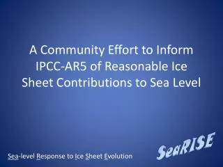
SeaRISE project aims to quantify upper-bound estimates of ice sheet contributions to sea level rise, utilizing ensemble modeling and data analysis. The project involves various ice sheet models and regional interactions to provide spatial detail and inform global climate models.

E N D
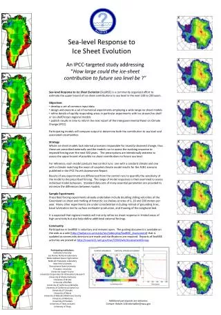
SeaRISE(Sea-level Response to Ice Sheet Evolution) “How bad could sea level rise get?”
Participants • Robert Bindschadler (NASA GSFC) • Ayako Abe-Ouchi (U. Tokyo) • Andy Aschwanden (ETH) • Richard Alley (Penn State) • Jeremy Bassis (U. Chicago) • Ed Bueler (UAF) • Bea Csatho (U Buffalo) • Mike Dinniman (Old Dominion) • Todd Dupont (UC Irvine) • Jim Fastook (U. Maine) • Carl Gladish (NYU/Courant) • Dan Goldberg (NYU/Courant/GFDL) • Ralf Greve (LTI/Hokaido) • David Holland (NYU/Courant) • Paul Holland (BAS) • Saffia Hossainzadeh (UC Santa Cruz) • Christina Hulbe (Portland State) • Charles Jackson (UTIG) • Jesse Johnson (U. Mont.) • John Klinck (Old Dominion) • Constantine Khroulev (UAF) • Anders Levermann (Potsdam) • Bill Lipscomb (LANL) • Doug MacAyeal (U. Chicago) • Maria Martin (Potsdam) • Sophie Nowicki (NASA) • Byron Parizek (Penn State) • David Pollard (Penn State) • Steve Price (LANL) • Catherine Ritz (LGGE) • Fuyuki Saito (Japan) • Olga Sergienko (Portland State) • Miren Vizcaino Trueba (UC Berkeley) • Slawek Tulaczyk (UC Santa Cruz) • Kees van der Veen (KU/CReSIS) • Ryan Walker (Penn State) • Weili Wang (NASA GSFC)
Origins • IPCC AR4 (of course) • “ability to predict dynamic ice sheet response is lacking” • Los Alamos Workshop (August 2008) on Incorporating Dynamic Ice Sheets into Global Climate Models • CCSM is on path to couple advanced-physics ice sheet to NCAR climate model • Not fast enough for IPCC AR5 • glaciological community input to 5th IPCC assessment is necessary
Goal • Provide quantitative upper-bound estimates of ice sheet contributions to sea level for the 21st century • complements Ice2Sea • SeaRISE also will: • Strengthen the ice sheet modeling community • Attract new individuals to ice sheet modeling • Facilitate integration of dynamic land ice into global climate models
Strategy • Identify upper bound of future sea-level rise and work toward increasing likelihood scenarios • Experiments replace missing physics by external forcings • e.g., start with removing all Antarctic ice shelves; prescribe subglacial lubrication; requireretreat/thinning of selected Greenland outlet glaciers • Multiple models • “Everyone” is more right than any “one” • Ensemble mean interpreted as a rough measure of uncertainty • Use common “best” data sets to remove these as source of model-to-model variations • SeaRISE is NOT a model intercomparison project
Participating Whole Ice Sheet Models • CISM/CCSM (built on GLIMMER) • PISM • Penn State U • U Maine • SICOPOLIS • GLAM • ICIES • GSFC • LGGE Each starts from its own control run with varying “spin-up” approaches
Regional models are involved too • 2-way interaction • Initialized from control runs of whole ice sheet models to provide spatial detail • Inform the whole ice sheet models through forcing boundary conditions, e.g., prescribe: • rate of grounding line retreat; • changing ice shelf backpressure; • perimeter thinning • basal lubrication from surface meltwater
Regional Models Type 1: Ice-Stream/Ice-Shelf • 2D or greater • Hulbe • Goldberg • Bassis (2.25-2.5D; an inverse approach) • Price/Payne (GLAM) • 1D,2D • Dupont • Parizek (no thermodynamics) • Price/Payne (GLAM run as vertical slice in the x,z plane)
Regional Models Type 2:Ice-Shelf/Ocean • 3D • HYPOP and CISM (Los Alamos National Lab; Ringler/Price/Lipscomb • ROMS (Old Dominion University; Klinck/Dinniman; no dynamical ice yet) • HIM (Ocean) (Geophysical Fluids Dynamics Lab; Little; no dynamical ice yet) • MICOM (Ocean) and CISM (University of Bergen ; Drange) • FESOM (Ocean) (Alfred Wegener Institute; Hellmer; and Hadley Center Ice Sheet) • 2D-Vertical • HYPOP and CISM (Los Alamos National Lab; Ringler/Price/Lipscomb • Stream Function Ocean Flowline Ice (Penn State University; Walker/Dupont; includes an ice stream) • 2D-Horizontal • Plume Ocean, CISM (New York University; Gladish/D.Holland; British Antarctic Survey; P.Holland; and Los Alamos National Lab; Lipscomb)
Data Sets Available at U/Montana Surface Elevation Bed Elevation Ice Thickness • Present day Antarctica data sets: • Mean Annual Surface Temperature • Ice Thickness • Accumulation/Ablation Rate • Ice Surface Elevation • Bed Topography • Basal Heat Flux • Thickness Mask • Surface Velocity • Melt(Ross ice streams) • Surface Balance Velocity • Present day Greenland data sets: • Ice Thickness • Bed Topography • Ice Surface Elevation • Precipitation • Basal Heat Flux • Mean Annual Near-surface(2m) Air Temperature Surface Temperature Precipitation Geothermal Heat Flow Balance Velocity
t0 = January 1, 2004 • Model simulations of present vary • experiment outputs will be compared to control runs of same model Surface Elevation minus Observed Basal Temperature
Control Runs • Constant Climate • hold climate constant at present values for 200 years (500 years preferred) • AR4 Climate • Use climate anomalies defined as ensemble mean of IPCC-AR4 models (provided by Tom Bracegirdle/BAS) • Standard output format has been defined to facilitate comparison analysis • Runs to be completed by November 30, 2009
Experiments • Scenario “experiments” are compared to a model’s own control run • Comparison of experiment anomalies minimizes model “peculiarities” • Greenland • Strong basal lubrication (and basal thawing) from surface meltwater • Prescribed glacier retreat/thinning • Antarctica • Ice-shelf removal • Estimate 2 experiments per year per ice sheet (including analysis, workshop and discussion)
Interaction • Bi-monthly telecoms • Bi-annual workshops • CCSM workshop (June) • Land Ice Working Group (February)
http://oceans11.lanl.gov/trac/CISM/wiki/AssessmentGroup http://websrv.cs.umt.edu/isis/index.php/Main_Page
Timetable • IPCC-AR5 will be finalized in 2014 • Published input likely due by 2Q/2012 • Control runs complete 4Q/2009 • 1st set of experiments complete by 1Q/2010 • Review results and define 2nd set of experiments by 2Q/2010 • Regional models generate prescribed forcing fields • 2nd set of experiments complete by 4Q/2010 • Possible 3rd round of experiments in 2011 • Review results and write papers by 1Q/2012