Lecture 3 The Gaussian Probability Distribution Function
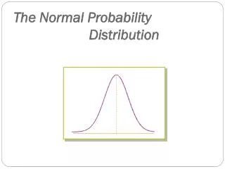
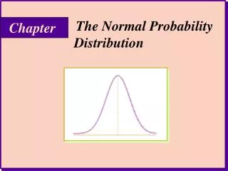
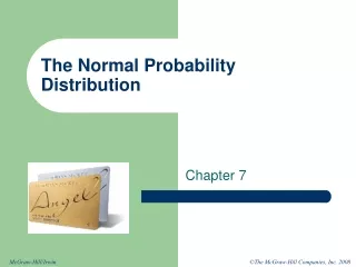
Lecture 3 The Gaussian Probability Distribution Function. Introduction l The Gaussian probability distribution is perhaps the most used distribution in all of science. Sometimes it is called the “bell shaped curve” or normal distribution.


Lecture 3 The Gaussian Probability Distribution Function
E N D
Presentation Transcript
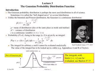
Lecture 3The Gaussian Probability Distribution Function Introduction l The Gaussian probability distribution is perhaps the most used distribution in all of science. Sometimes it is called the “bell shaped curve” or normal distribution. l Unlike the binomial and Poisson distribution, the Gaussian is a continuous distribution: = mean of distribution (also at the same place as mode and median) 2 = variance of distribution y is a continuous variable (-∞y∞ l Probability (P) of y being in the range [a, b] is given by an integral: u The integral for arbitrary a and b cannot be evaluated analytically. The value of the integral has to be looked up in a table (e.g. Appendixes A and B of Taylor). Karl Friedrich Gauss 1777-1855 The integrals with limits [-¥, ¥] can be evaluated, see Barlow P. 37. Plot of Gaussian pdf p(x) x P416 Lec 3
l The total area under the curve is normalized to one by the σ√(2π) factor. l We often talk about a measurement being a certain number of standard deviations () away from the mean () of the Gaussian. We can associate a probability for a measurement to be |- n| away from the mean just by calculating the area outside of this region. n Prob. of exceeding m±n 0.67 0.5 1 0.32 2 0.05 3 0.003 4 0.00006 It is very unlikely (< 0.3%) that a measurement taken at random from a Gaussian pdf will be more than ± 3s from the true mean of the distribution. Gaussian pdf with m=0 and s=1 95% of area within 2s Only 5% of area outside 2s P416 Lec 3
Relationship between Gaussian and Binomial & Poisson distribution The Gaussian distribution can be derived from the binomial (or Poisson) assuming: p is finite & N is very large we have a continuous variable rather than a discrete variable Consider tossing a coin 10,000 times. p(head) = 0.5 and N = 10,000 For a binomial distribution: mean number of heads = = Np = 5000 standard deviation = [Np(1 - p)]1/2 = 50 The probability to be within m±1for this binomial distribution is: For a Gaussian distribution: Both distributions give about the ~ same probability! See Taylor10.4 Compare ±1σ area of Poisson and Gaussian: Mean Poission Gaussian % diff 10 0.74 0.6827 7.8 25 0.73 0.6827 6.9 100 0.707 0.6827 3.5 250 0.689 0.6827 0.87 5000 0.6847 0.6827 0.29 P416 Lec 3
Why is the Gaussian pdf so applicable? Þ Central Limit Theorem A crude statement of the Central Limit Theorem: Things that are the result of the addition of lots of small effects tend to become Gaussian. A more exact statement: Let Y1, Y2,...Yn be an infinite sequence of independent random variables each with the same probability distribution. Suppose that the mean () and variance (2) of this distribution are both finite. For any numbers a and b: The C.L.T. tells us that under a wide range of circumstances the probability distribution that describes the sum of random variables tends towards a Gaussian distribution as the number of terms in the sum ∞. Actually, the Y’s can be from different pdf’s! How close to ¥ does n have to be?? Alternatively we can write the CLT in a different form: P416 Lec 3
—m is sometimes called “the error in the mean” (more on that later): FFor CLT to be valid: • The m and s of the pdf must be finite. • No one term in sum should dominate the sum. • lA random variable is not the same as a random number. • “A random variable is any rule that associates a number with each outcome in S” • (Devore, in “probability and Statistics for Engineering and the Sciences”). • Here S is the set of possible outcomes. • l Recall if y is described by a Gaussian pdf with mean (m) of zero and s=1 then the probability that a<y<b is given by: • The CLT is true even if the Y’s are from different pdf’s as long as the means • and variances are defined for each pdf ! • See Appendix of Barlow for a proof of the Central Limit Theorem. P416 Lec 3
lExample: Generate a Gaussian distribution using uniform random numbers. u Random number generator gives numbers distributed uniformly in the interval [0,1] nm= 1/2 and s2 = 1/12 u Procedure: a) Take 12 numbers (r1, r2,……r12) from your computer’s random number generator (ran(iseed)) b) Add them together c) Subtract 6 Þ Get a number that looks as if it is from a Gaussian pdf! A) 5000 random numbers B) 5000 pairs (r1 + r2) of random numbers D) 5000 12-plets (r1 + r2 +…r12) of random numbers. C) 5000 triplets (r1 + r2 + r3) of random numbers E) 5000 12-plets (r1 + r2 +…r12 - 6)of random numbers. E Gaussian m= 0 and s= 1 Thus the sum of 12 uniform random numbers minus 6 is distributed as if it came from a Gaussian pdf with m = 0 and s= 1. -6 0 +6 12 is close to ¥ !! P416 Lec 3
·Example: A watch makes an error of at most ±1/2 minute per day. After one year, what’s the probability that the watch is accurate to within ±25 minutes? • u Assume that the daily errors are uniform in [-1/2, 1/2]. • n For each day, the average error is zero and the standard deviation 1/√12 minutes. • n The error over the course of a year is just the addition of the daily error. • n Since the daily errors come from a uniform distribution with a well defined mean and variance the Central Limit Theorem is applicable: • The upper limit corresponds to +25 minutes: • The lower limit corresponds to –25 minutes. • The probability to be within±25 minutes is: • The probability to be offby more than 25 minutes is just: 1-P»1-0.999997=3´10-6 • There is < 3 in a million chance that the watch will be off by more than 25 minutes in a year! This integral is ≈ 1 to about 3 part in 106! P416 Lec 3
l Example: The daily income of a “card shark” has a uniform distribution in the interval [-$40,$50]. What is the probability that s/he wins more than $500 in 60 days? u Lets use the CLT to estimate this probability: u The probability distribution of daily income is uniform, p(y) = 1. p(y) needs to be normalized in computing the average daily winning () and its standard deviation (). • u The lower limit of the winnings is $500: • u The upper limit is the maximum that the shark could win (50$/day for 60 days): 16% chance to win $500 in 60 days P416 Lec 3