Probability Distribution

1. Probability Distribution Sec: 6.1

2. New Vocabulary: • Random Variable; • A random variable is the numerical measurement of the outcomes of a random phenomenon. • Examples: • Role of a die • Drawing cards • Work hours of randomly selected person • Score of a random game of soccer • A pass or fail mark for a random student

3. Notation: • We will use capital letters to refer to the random variable itself; • X is the number of heads from three coins • Y is the flight speed of an unladen swallow • We will use lower case letters to refer to specific values of the variable; • x=2, for two heads • y=32.4 mph for a selected swallow

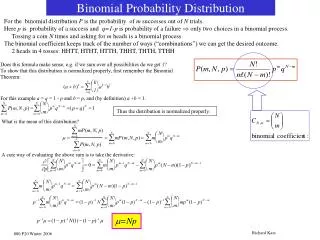
4. Probability Distribution: • As the outcome to a random Phenomenon each value of the random variable has a specific probability. • An organized collection of these probabilities forms a probability distribution, Denoted P(x). • Give the distribution the value(s) you want and it will tell you the probability of those values occurring. • Example: P(4)=0.23 means there is a 23% chance of a four as an outcome.

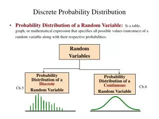
5. Note on Probability Distributions • P(x) is between 0 and 1 for any x. • The sum of all values for P(x) is 1 • Example: Let X= the role of a fair die. • Then P(1)=P(2)=P(3)=P(4)=P(5)=P(6)=1/6 • And 1/6+1/6+1/6+1/6+1/6+1/6=1 • Random variables can be discrete or continuous. Uniform distribution!

6. Example: • The probability distribution for the number of years left until students get he degree they seek is given in the table. • Question: • Does this meet both criteria for a probability distribution? • What is the Probability that a selected student has one year left? • What is the probability that a student has more the one year left? • Can we graph this

7. Histogram for Probability Distribution: Skew?

8. Descriptive Statistics: • Like our other number sets the probability distribution has central tendencies, spread. As before we can use mean and standard deviation to describe this center and spread. • With one big difference. • Because our probabilities are values for the population these measures are considered parameters. • For parameters we use Greek letters so we can differentiate from statistics. • We use μ for the mean, (Mu, pronounced “Mew”) • We use σ for standard deviation, (sigma)

9. Finding μ: Recall: To find the mean we need to add up all the values and divide by the number of values that occur. But how many values are there? How can we make this work? According to our table we will have 21 out of 100 students that have half a year left, 31 of 100 with one year left, and so on. We can find μ by letting the number of values be equal to 100 and use the percentages as the number of times they occur. So, the Average student has 1.31 years left until they get there degree.

10. Finding μ, a better way; • Lets simplify this, • We do not need to turn the probabilities into percents to only divide by 100 while finding the mean. We can simply multiply the outcomes by their correct probabilities, their sum will be our mean. • This is often called a weighted average • This is often called the expected value.

11. Expected Value; • Let’s play a game. • You give me one dollar. I role a die. • On a 1,2, or 3, you get nothing back. • On a 4, or 5, you get 25 cents back. • On a six you get five dollars. • Do you want to play?

12. Do we want to play? • Step one: The sample space. • We could get zero, 25 cents, or five dollars. • Step two the probabilities. • 3 in 6 for zero back • 2 in 6 for 25 cents • 1 in 6 for five dollars • Step three: Find μ, • 0(1/2)+.25(1/3)+5(1/6)=0.92 • Should we play?

13. Questions? Anyone?

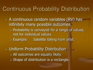
14. Continuous Random Variables: • For continuous variables we find the probability of values occurring within an interval instead of at individual points. • For Example for heights we often round to the nearest inch. Therefore 68 inches tall actually represents the interval from 67.5 inches to 68.5 inches. • The smaller the intervals, and larger the sample, the closer we will get to the ideal distribution. • Like discrete distributions the probability of any interval is between 0 and 1 and the probability of the whole interval is one.

15. Continuous Random Variables: With few intervals the graphs will be wrought even will a large sample. But as the intervals shrink the graph will become increasingly smooth. Until finally becoming the smooth curve.

16. Probability and area: The probability of an interval is equal to the area under the curve over that interval. Area=.15 units P(A)=.15 = 15% A

17. Probability and area: What is the area under the whole curve? P(B) = 1 Area = 1 unit B

18. Probability and area: It is uncommon for data to be perfectly normal. Either the data comes from to small of a sample, or the discrete intervals make the image jagged, or the data was just never normal to begin with. We will however use the normal curve for many of our models that are “nearly” normal. It is simply to powerful of a tool to worry about it fitting “just right”. And we can get surprisingly accurate results from distributions that are quite a bit off from normal. We just need to be careful and aware.

19. Next Time: Binomials HW: 6.1; 6, 19*, 23*, 27, 31,33