Download
1 / 25
300 likes | 825 Views
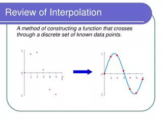
Review of Interpolation. A method of constructing a function that crosses through a discrete set of known data points. . . Spline (general case). Given n +1 distinct knots x i such that:. with n +1 knot values y i find a spline function.

E N D
Review of Interpolation A method of constructing a function that crosses through a discrete set of known data points. .
Spline (general case) • Given n+1 distinct knotsxi such that: with n+1 knot values yi find a spline function with each Si(x) a polynomial of degree at most n.
Spline Interpolation • Linear, Quadratic, Cubic • Preferred over other polynomial interpolation • More efficient • High-degree polynomials are very computationally expensive • Smaller error • Interpolant is smoother
Natural Cubic Spline Interpolation • Si(x) = aix3 + bix2 + cix + di • 4 Coefficients with n subintervals = 4n equations • There are 4n-2 conditions • Interpolation conditions • Continuity conditions • Natural Conditions • S’’(x0) = 0 • S’’(xn) = 0
Bezier Curves • A similar but different problem: Controlling the shape of curves. Problem: given some (control) points, produce and modify the shape of a curve passing through the first and last point. http://www.ibiblio.org/e-notes/Splines/Bezier.htm
Bezier Curves Idea: Build functions that are combinations of some basic and simpler functions. Basic functions: B-splines Bernstein polynomials
Bernstein Polynomials • Bernstein polynomials of degree n are defined by: • For v = 0, 1, 2, …, n, • In general there are N+1 Bernstein Polynomials of degree N. For example, the Bernstein Polynomials of degrees 1, 2, and 3 are: • 1. B0,1(t) = 1-t, B1,1(t) = t; • 2. B0,2(t) = (1-t)2, B1,2(t) = 2t(1-t), B2,2(t) = t2; • 3. B0,3(t) = (1-t)3, B1,3(t) = 3t(1-t)2, B2,3(t)=3t2(1-t), B3,3(t) = t3;
Deriving the Basis Polynomials • Write 1 = t + (1-t) and raise 1 to the third power for cubic splines (2 for quadratic, 4 for quartic, etc…) • 1^3 = (t + (1-t))^3 = t^3 + 3t^2(1-t) + 3t(1-t)^2 + (1-t)^3 • The basis functions are the four terms: • B0(t) = (1-t)^3 • B1(t) = 3t(1-t)^2 • B2(t) = 3t^2(1-t) • B3(t) = t^3
Bernstein Polynomials Bernstein polynomials of degree 3
Using the Basis Functions • To use the Bernstein basis functions to make a spline we need 4 “control” points for a cubic. (3 for quadratic, 5 for quartic, etc…) • Let (x0,y0), (x1,y1), (x2,y2), (x3,y3) be the “control”points • The x and y coordinates of the cubic Bezier spline are given by: • x(t) = x0B0(t) + x1B1(t) +x2B2(t) + x3B3(t) • y(t) = y0B0(t) + y1B1(t) + y2B2(t) + y3B3(t) • Where 0<= t <= 1.
Bernstein Polynomials • Given a set of control points {Pi}Ni=0, where Pi = (xi, yi). A Bezier curve of degree N is: P(t) = Ni=0 PiBi,N(t), • Where Bi,N(t), for I = 0, 1, …, N, are the Bernstein polynomials of degree N. • P(t) is the Bezier curve Since Pi = (xi, yi) • x(t) = Ni=0xiBi,N(t) and y(t) = Ni=0yiBi,N(t) • The spline goes through (x0,y0) and (x3,y3) • The tangent at those points is the line connecting (x0,y0) to (x1,y1) and (x3,y3) to (x2,y2). • The positions of (x1,y1) and (x2,y2) determine the shape of the curve.
Bernstein Polynomials Example • Find the Bezier curve which has the control points (2,2), (1,1.5), (3.5,0), (4,1). Substituting the x- and y-coordinates of the control points and N=3 into the x(t) and y(t) formulas on the previous slide yields x(t) = 2B0,3(t) + 1B1,3(t) + 3.5B2,3(t) + 4B3,3(t) y(t) = 2B0,3(t) + 1.5B1,3(t) + 0B2,3(t) + 1B3,3(t)
Bernstein Polynomials Example • Substitute the Bernstein polynomials of degree three into these formulas to get x(t) = 2(1 – t)3 + 3t(1 – t)2 + 10.5t2(1 – t) + 4t3 y(t) = 2(1-t)3 + 4.5t(1 – t)2 + t3 • Simplify these formulas to yield the parametric equation: P(t) = (2 – 3t + 10.5t2 – 5.5t3, 2 – 1.5t – 3t2 + 3.5t3) where 0 < t < 1 P(t) is the Bezier curve http://www.cs.brown.edu/exploratories/freeSoftware/repository/edu/brown/cs/exploratories/applets/bezierSplines/bezier_splines_java_browser.html
Composite Bezier Curves • In practice, shapes are often constructed of multiple Bezier curves combined together. • Allows for flexibility in constructing shapes. (Consecutive Bezier curves need not join smoothly.)
Composite Bezier Curves • Linking curves: • Example: Find the composite Bezier curve for the four sets of control points: {(-9,0), (-8,1), (-8,2.5), (-4,2.5)}, {(-4,2.5), (-3,3.5), (-1,4), (0,4)} {(0,4), (2,4), (3,4), (5,2)}, {(5,2), (6,2), (20,3), (18,0)}
Composite Bezier Curves Use the same process as earlier to yield these four parametric equations: • P1(t) = (-9 + 3t - 3t2 + 5t3, 3t + 1.5t2 - 2t3) • P2(t) = (-4 + 3t + 3t2 - 2t3, 2.5 + 3t - 1.5t2) • P3(t) = (6t - 3t2 + 2t3, 4 - 2t3) • P4(t) = (5 + 3t + 39t2 - 29t3, 2 + 3t2 - 5t3)
Composite Bezier Curves Linking Curves Smoothly • To have two Bezier curves P(t) and Q(t) meet smoothly would require: • PN = Q0 • P’(PN) = Q’(Q0) • It is sufficient to require that the control points PN-1, PN = Q0, and Q1 be collinear.
Composite Bezier Curves • Example of collinear control points: {(0,3), (1,5), (2,1), (3,3)} and {(3,3), (4,5), (5,1), (6,3)} P(t) = (3t, 3 + 6t - 18t2 + 12t3) Q(t) = (3 + 3t, 3 + 6t – 18t2 + 12t3) and P’(t) = (3, 6 – 36t + 36t2) Q’(t) = (3, 6 – 36t + 36t2) Substituting t = 1 and t = 0 into P’(t) and Q’(t), yields P’(1) = (3,6) = Q’(0)
Composite Bezier Curves It’s collinear!
1.900 0.850 1.900 0.850 1.900 0.700 1.900 0.700 1.900 0.850 1.850 0.930 1.800 0.950 1.666 0.950 1.333 0.050 1.333 0.050 1.666 0.050 1.666 0.050 1.100 0.800 1.120 0.910 1.200 0.950 1.333 0.950 1.100 0.800 1.100 0.800 1.100 0.200 1.100 0.200 1.100 0.200 1.120 0.090 1.200 0.050 1.333 0.050 1.333 0.950 1.333 0.950 1.666 0.950 1.666 0.950 1.900 0.150 1.850 0.070 1.800 0.050 1.666 0.050 1.900 0.150 1.900 0.150 1.900 0.300 1.900 0.300 1.900 0.700 1.900 0.700 1.780 0.700 1.780 0.700 1.780 0.700 1.780 0.780 1.720 0.820 1.600 0.820 1.780 0.300 1.780 0.220 1.720 0.180 1.600 0.180 1.200 0.700 1.200 0.700 1.200 0.300 1.200 0.300 1.600 0.820 1.600 0.820 1.333 0.820 1.333 0.820 1.600 0.180 1.600 0.180 1.333 0.180 1.333 0.180 1.333 0.180 1.230 0.180 1.200 0.230 1.200 0.300 1.333 0.820 1.230 0.820 1.200 0.770 1.200 0.700 1.780 0.300 1.780 0.300 1.600 0.300 1.600 0.300 1.600 0.300 1.600 0.300 1.600 0.370 1.600 0.370 1.600 0.370 1.600 0.370 1.950 0.370 1.950 0.370 1.950 0.370 1.950 0.370 1.950 0.300 1.950 0.300 1.950 0.300 1.950 0.300 1.900 0.300 1.900 0.300 Practical Applications • 0.900 0.850 0.900 0.850 0.900 0.700 0.900 0.700 • 0.900 0.850 0.850 0.930 0.800 0.950 0.666 0.950 • 0.333 0.050 0.333 0.050 0.666 0.050 0.666 0.050 • 0.100 0.800 0.120 0.910 0.200 0.950 0.333 0.950 • 0.100 0.800 0.100 0.800 0.100 0.200 0.100 0.200 • 0.100 0.200 0.120 0.090 0.200 0.050 0.333 0.050 • 0.333 0.950 0.333 0.950 0.666 0.950 0.666 0.950 • 0.900 0.150 0.850 0.070 0.800 0.050 0.666 0.050 • 0.900 0.150 0.900 0.150 0.900 0.300 0.900 0.300 • 0.900 0.700 0.900 0.700 0.780 0.700 0.780 0.700 • 0.780 0.700 0.780 0.780 0.720 0.820 0.600 0.820 • 0.900 0.300 0.900 0.300 0.780 0.300 0.780 0.300 • 0.780 0.300 0.780 0.220 0.720 0.180 0.600 0.180 • 0.200 0.700 0.200 0.700 0.200 0.300 0.200 0.300 • 0.600 0.820 0.600 0.820 0.333 0.820 0.333 0.820 • 0.600 0.180 0.600 0.180 0.333 0.180 0.333 0.180 • 0.333 0.180 0.230 0.180 0.200 0.230 0.200 0.300 • 0.333 0.820 0.230 0.820 0.200 0.770 0.200 0.700
Practical Applications • 4.35 0.00 4.35 0.00 4.35 0.19 4.35 0.19 • 4.35 0.19 3.53 0.23 3.39 0.36 3.39 1.09 • 3.39 1.09 3.39 1.08 3.39 6.20 3.39 6.20 • 3.39 6.20 3.39 6.20 3.93 6.20 3.93 6.20 • 3.93 6.20 5.07 6.20 5.29 6.02 5.52 4.92 • 5.52 4.92 5.52 4.92 5.76 4.92 5.76 4.92 • 5.76 4.92 5.76 4.92 5.70 6.62 5.70 6.62 • 5.70 6.62 5.70 6.62 0.30 6.62 0.30 6.62 • 0.24 4.92 0.24 4.92 0.30 6.62 0.30 6.62 • 0.48 4.92 0.48 4.92 0.24 4.92 0.24 4.92 • 2.07 6.20 0.93 6.20 0.71 6.02 0.48 4.92 • 2.61 6.20 2.61 6.20 2.07 6.20 2.07 6.20 • 2.61 1.09 2.61 1.08 2.61 6.20 2.61 6.20 • 1.65 0.19 2.47 0.23 2.61 0.36 2.61 1.09 • 1.65 0.00 1.65 0.00 1.65 0.19 1.65 0.19 • 1.65 0.00 1.65 0.00 4.35 0.00 4.35 0.00