Multiple Regression

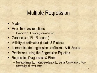
1. Multiple Regression • Model • Error Term Assumptions • Example 1: Locating a motor inn • Goodness of Fit (R-square) • Validity of estimates (t-stats & F-stats) • Interpreting the regression coefficients & R-Square • Predictions using the Regression Equation • Regression Diagnostics & Fixes • Multicollinearity, Heteroskedasticity, Serial Correlation, Non-normality of error term

2. Introduction • In this model we extend the simple linear regression model, and allow for any number of independent variables. • We will also learn to detect econometric problems.

3. Dependent variable Independent variables Model and Required Conditions • We allow for k independent variables to potentially be related to the dependent variable y = b0 + b1x1+ b2x2 + …+ bkxk + e Coefficients Random error variable

4. The simple linear regression model allows for one independent variable, “x” y =b0 + b1x + e y y = b0 + b1x y = b0 + b1x y = b0 + b1x y = b0 + b1x Note how the straight line becomes a plain, and... y = b0 + b1x1 + b2x2 y = b0 + b1x1 + b2x2 y = b0 + b1x1 + b2x2 y = b0 + b1x1 + b2x2 y = b0 + b1x1 + b2x2 X y = b0 + b1x1 + b2x2 1 y = b0 + b1x1 + b2x2 The multiple linear regression model allows for more than one independent variable. Y = b0 + b1x1 + b2x2 + e X2

5. Required conditions for the error variable e • The error e is normally distributed with mean equal to zero and a constant standard deviation se(independent of the value of y). se is unknown. • The errors are independent. • These conditions are required in order to • estimate the model coefficients, • assess the resulting model.

6. Example 1 Where to locate a new motor inn? • La Quinta Motor Inns is planning an expansion. • Management wishes to predict which sites are likely to be profitable. • Several areas where predictors of profitability can be identified are: • Competition • Market awareness • Demand generators • Demographics • Physical quality

7. Physical Margin Profitability Competition Market awareness Customers Community Rooms Nearest Office space College enrollment Income Disttwn Median household income. Number of hotels/motels rooms within 3 miles from the site. Distance to the nearest La Quinta inn. Distance to downtown.

8. Data was collected from randomly selected 100 inns that belong to La Quinta, and ran for the following suggested model: Margin =b0 + b1Rooms + b2Nearest + b3Office + b4College + b5Income + b6Disttwn +

9. This is the sample regression equation (sometimes called the prediction equation) MARGIN = 72.455 - 0.008ROOMS-1.646NEAREST + 0.02OFFICE +0.212COLLEGE - 0.413INCOME + 0.225DISTTWN • Excel output Let us assess this equation

10. Standard error of estimate • We need to estimate the standard error of estimate • Compare seto the mean value of y • From the printout, Standard Error = 5.5121 • Calculating the mean value of y we have • It seems se is not particularly small. • Can we conclude the model does not fit the data well?

11. Coefficient of determination • The definition is • From the printout, R2 = 0.5251 • 52.51% of the variation in the measure of profitability is explained by the linear regression model formulated above. • When adjusted for degrees of freedom, Adjusted R2 = 1-[SSE/(n-k-1)] / [SS(Total)/(n-1)] = = 49.44%

12. Testing the validity of the model • We pose the question: Is there at least one independent variable linearly related to the dependent variable? • To answer the question we test the hypothesis H0: b1 = b2 = … = bk = 0 H1: At least one bi is not equal to zero. • If at least one bi is not equal to zero, the model is valid.

13. MSR = F MSE • To test these hypotheses we perform an analysis of variance procedure. • The F test • Construct the F statistic • Rejection region F>Fa,k,n-k-1 MSR=SSR/k [Variation in y] = SSR + SSE. Large F results from a large SSR. Then, much of the variation in y is explained by the regression model. The null hypothesis should be rejected; thus, the model is valid. MSE=SSE/(n-k-1) Required conditions must be satisfied.

14. y Two data points (x1,y1) and (x2,y2) of a certain sample are shown. y2 y1 x1 x2 Total variation in y = Variation explained by the regression line) + Unexplained variation (error)

15. Example 1 - continued • Excel provides the following ANOVA results MSR/MSE MSE SSE MSR SSR

16. Example 1 - continued • Excel provides the following ANOVA results Conclusion: There is sufficient evidence to reject the null hypothesis in favor of the alternative hypothesis. At least one of the bi is not equal to zero. Thus, at least one independent variable is linearly related to y. This linear regression model is valid Fa,k,n-k-1 = F0.05,6,100-6-1=2.17 F = 17.14 > 2.17 Also, the p-value (Significance F) = 3.03382(10)-13 Clearly, a = 0.05>3.03382(10)-13, and the null hypothesis is rejected.

17. Let us interpret the coefficients • This is the intercept, the value of y when all the variables take the value zero. Since the data range of all the independent variables do not cover the value zero, do not interpret the intercept. • In this model, for each additional 1000 rooms within 3 mile of the La Quinta inn, the operating margin decreases on the average by 7.6% (assuming the other variables are held constant).

18. In this model, for each additional mile that the nearest competitor is to La Quinta inn, the average operating margin decreases by 1.65% • For each additional 1000 sq-ft of office space, the average increase in operating margin will be .02%. • For additional thousand students MARGIN increases by .21%. • For additional $1000 increase in median household income, MARGIN decreases by .41% • For each additional mile to the downtown center, MARGIN increases by .23% on the average

19. H0: bi = 0 H1: bi = 0 Test statistic • Testing the coefficients • The hypothesis for each bi • Excel printout d.f. = n - k -1

20. Using the linear regression equation • The model can be used by • Producing a prediction interval for the particular value of y, for a given set of values of xi. • Producing an interval estimate for the expected value of y, for a given set of values of xi. • The model can be used to learn about relationships between the independent variables xi, and the dependent variable y, by interpreting the coefficients bi

21. Example 1 - continued. Produce predictions • Predict the MARGIN of an inn at a site with the following characteristics: • 3815 rooms within 3 miles, • Closet competitor 3.4 miles away, • 476,000 sq-ft of office space, • 24,500 college students, • $39,000 median household income, • 3.6 miles distance to downtown center. MARGIN = 72.455 - 0.008(3815)-1.646(3.4) + 0.02(476) +0.212(24.5) - 0.413(39) + 0.225(3.6) = 37.1%

22. Regression Diagnostics - II • The required conditions for the model assessment to apply must be checked. • Is the error variable normally distributed? (JB Stat) • Is the error variance constant? (White Test) • Are the errors independent? (DW Test) • Can we identify outliers? • Is multicollinearity a problem?

23. Example 2 House price and multicollinearity • A real estate agent believes that a house selling price can be predicted using the house size, number of bedrooms, and lot size. • A random sample of 100 houses was drawn and data recorded. • Analyze the relationship among the four variables

24. Solution • The proposed model isPRICE = b0 + b1BEDROOMS + b2H-SIZE +b3LOTSIZE + e • Excel solution The model is valid, but no variable is significantly related to the selling price !!

25. However, • when regressing the price on each independent variable alone, it is found that each variable is strongly related to the selling price. • Multicollinearity is the source of this problem. • Multicollinearity causes two kinds of difficulties: • The t statistics appear to be too small. • The b coefficients cannot be interpreted as “slopes”.

26. ^ y + + + + + + + + + + + + + + + + + + + + + + + + + + + + + + + + + + + + + + + + + + + + • When the requirement of a constant variance is met we have homoscedasticity. Residual + + + + + + + + + + + + + + ^ + + y + + + + + + + + The spread of the data points does not change much.

27. ^ y + + + + + + + + + + + + + + + + + + + + + + + ^ The spread increases with y Heteroscedasticity • When the requirement of a constant variance is violated we have heteroscedasticity. The plot of the residual Vs. predicted value of Y will exhibit a cone shape. Residual + + + + + + + + + + + + + ^ + + + y + + + + + + + +

28. Detection/ Fix for Heteroscedasticity • Detection: White test (Use Chi-square stat) • Fix: White Correction (Uses OLS but keeps heteroscedasticity from making the variance of the OLS estimators swell in size)

29. Patterns in the appearance of the residuals over time indicates that autocorrelation exists. Residual Residual + + + + + + + + + + + + + + 0 0 Time Time + + + + + + + + + + + + + + Note the runs of positive residuals, replaced by runs of negative residuals Note the oscillating behavior of the residuals around zero.

30. Positive first order autocorrelation occurs when consecutive residuals tend to be similar. Then, the value of d is small (less than 2). Positive first order autocorrelation + Residuals + + + 0 Time + + + + Negative first order autocorrelation Negative first order autocorrelation occurs when consecutive residuals tend to markedly differ. Then, the value of d is large (greater than 2). Residuals + + + 0 + + Time + +

31. Autocorrelation or Serial Correlation • The Durbin - Watson Test • This test detects first order auto-correlation between consecutive residuals in a time series • If autocorrelation exists the error variables are not independent Residual at time i

32. One tail test for positive first order auto-correlation • If d<dL there is enough evidence to show that positive first-order correlation exists • If d>dU there is not enough evidence to show that positive first-order correlation exists • If d is between dL and dU the test is inconclusive. • One tail test for negative first order auto-correlation • If d>4-dL, negative first order correlation exists • If d<4-dU, negative first order correlation does not exists • if d falls between 4-dU and 4-dL the test is inconclusive.

33. First order correlation does not exist First order correlation does not exist First order correlation exists Inconclusive test First order correlation exists Inconclusive test • Two-tail test for first order auto-correlation • If d<dL or d>4-dL first order auto-correlation exists • If d falls between dL and dU or between 4-dU and 4-dL the test is inconclusive • If d falls between dU and 4-dU there is no evidence for first order auto-correlation 0 dL dU 2 4-dU 4-dL 4

34. Example 3 • How does the weather affect the sales of lift tickets in a ski resort? • Data of the past 20 years sales of tickets, along with the total snowfall and the average temperature during Christmas week in each year, was collected. • The model hypothesized was TICKETS=b0+b1SNOWFALL+b2TEMPERATURE+e • Regression analysis yielded the following results:

35. The model seems to be very poor: • The fit is very low (R-square=0.12), • It is not valid (Signif. F =0.33) • No variable is linearly related to Sales Diagnosis of the required conditions resulted with the following findings

36. Residual vs. predicted y The error distribution The error variance is constant The errors may be normally distributed Residual over time The errors are not independent

37. Test for positive first order auto-correlation: n=20, k=2. From the Durbin-Watson table we have: dL=1.10, dU=1.54. The statistic d=0.59 Conclusion: Because d<dL , there is sufficient evidence to infer that positive first order auto-correlation exists. Using the computer - Excel Tools > data Analysis > Regression (check the residual option and then OK) Tools > Data Analysis Plus > Durbin Watson Statistic > Highlight the range of the residuals from the regression run > OK The residuals

38. The modified regression model TICKETS=b0+ b1SNOWFALL+ b2TEMPERATURE+ b3YEARS+e The autocorrelation has occurred over time. Therefore, a time dependent variable added to the model may correct the problem • All the required conditions are met for this model. • The fit of this model is high R2 = 0.74. • The model is useful. Significance F = 5.93 E-5. • SNOWFALL and YEARS are linearly related to ticket sales. • TEMPERATURE is not linearly related to ticket sales.

39. Non-normality of Error term • Indication of Non-normal Distribution: Mean quite different from median of residual. Skewness of residual is not zero. Kurtosis is much different than 3. (Formal test Jarque-Bera Test) • Fix: Transform the dependent variable. Log(y), Square Y, Square Root of Y, 1/Y etc.