Download
1 / 68
690 likes | 888 Views
Lecture 4 The L 2 Norm and Simple Least Squares. Syllabus.

E N D
Syllabus Lecture 01 Describing Inverse ProblemsLecture 02 Probability and Measurement Error, Part 1Lecture 03 Probability and Measurement Error, Part 2 Lecture 04 The L2 Norm and Simple Least SquaresLecture 05 A Priori Information and Weighted Least SquaredLecture 06 Resolution and Generalized Inverses Lecture 07 Backus-Gilbert Inverse and the Trade Off of Resolution and VarianceLecture 08 The Principle of Maximum LikelihoodLecture 09 Inexact TheoriesLecture 10 Nonuniqueness and Localized AveragesLecture 11 Vector Spaces and Singular Value Decomposition Lecture 12 Equality and Inequality ConstraintsLecture 13 L1 , L∞ Norm Problems and Linear ProgrammingLecture 14 Nonlinear Problems: Grid and Monte Carlo Searches Lecture 15 Nonlinear Problems: Newton’s Method Lecture 16 Nonlinear Problems: Simulated Annealing and Bootstrap Confidence Intervals Lecture 17 Factor AnalysisLecture 18 Varimax Factors, Empircal Orthogonal FunctionsLecture 19 Backus-Gilbert Theory for Continuous Problems; Radon’s ProblemLecture 20 Linear Operators and Their AdjointsLecture 21 Fréchet DerivativesLecture 22 Exemplary Inverse Problems, incl. Filter DesignLecture 23 Exemplary Inverse Problems, incl. Earthquake LocationLecture 24 Exemplary Inverse Problems, incl. Vibrational Problems
Purpose of the Lecture Introduce the concept of prediction error and the norms that quantify it Develop the Least Squares Solution Develop the Minimum Length Solution Determine the covariance of these solutions
The Linear Inverse Problem Gm = d
The Linear Inverse Problem Gm = d model parameters data data kernel
an estimate of the model parameters can be used to predict the data Gmest = dpre but the prediction may not match the observed data (e.g. due to observational error) dpre ≠ dobs
this mismatch leads us to define the prediction error e = dobs -dpre e = 0 when the model parameters exactly predict the data
example of prediction error for line fit to data B) A) diobs ei dipre zi
“norm”rule for quantifying the overall size of the error vector e lot’s of possible ways to do it
Ln family of norms Euclidian length
guiding principle for solving an inverse problemfind the mestthat minimizes E=||e||withe = dobs –dpreanddpre= Gmest
L1 L2 L∞ outlier
Answer is related to the distribution of the error. Are outliers common or rare? A) B) short tails outliers uncommon outliers important use high norm gives high weight to outliers long tails outliers common outliers unimportant use low norm gives low weight to outliers
as we will show later in the class … use L2 norm when data hasGaussian-distributed error
L2norm of error is its Euclidian length = eTe so E is the square of the Euclidean length mimimizeE Principle of Least Squares
Least Squares Solution to Gm=d minimize E with respect to mq ∂E/∂mq = 0
first term ∂mj /∂mq= δjq since mj and mqare independent variables
Kronecker delta(elements of identity matrix)[I]ij= δij a = Ib = b ai = Σjδijbj =bi ai = Σjδijbj =bi i
second term third term
presuming [GTG] has an inverse Least Square Solution
presuming [GTG] has an inverse Least Square Solution memorize
example straight line problem Gm = d
in practice,no need to multiply matrices analyticallyjust use MatLab mest = (G’*G)\(G’*d);
z, km y, km x, km
examplefitting line to a single point ? ? d ? z
Least Squares will failwhen more than one solution minimizes the errorthe inverse problem is “underdetermined”
What to do?use another guiding principle“a priori” information about the solution
simplest case“purely underdetermined”more than one solution has zero error
Method of Lagrange Multipliersminimize L with constraintsC1=0, C2=0, …equivalent tominimize Φ=L+λ1C1+λ2C2+…with no constraintsλs called “Lagrange Multipliers”
e(x,y)=0 y (x0,y0) L (x,y) x