Hyperspectral IR Cloudy Fast Forward Model

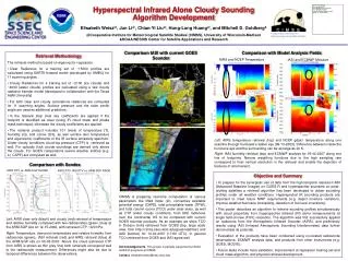
1. Hyperspectral IR Cloudy Fast Forward Model J. E. Davies, X. Wang, E. R. Olson, J. A. Otkin, H-L. Huang, Ping Yang#, Heli Wei#, Jianguo Niu# and David D. Turner* Cooperative Institute for Meteorological Satellite Studies (CIMSS), Madison, WI #Department of Atmospheric Sciences, Texas A&M University, College Station, TX*Climate Physics Group, Pacific Northwest National Laboratory, Richland, WA 99352 jimd@ssec.wisc.edu and/or xuanjiw@ssec.wisc.edu

2. Outline • Objective • Single-layer cloud model • Two-layer cloud model • Current status • Future work

3. Objective A rapid and accurate hyperspectral infrared clear and cloudy radiative transfer model is developed to simulate the Top-Of-Atmosphere (TOA) radiances and brightness temperatures over a broad spectral band (~3-100µm). The principal use of this effort is to generate TOA radiances over large spatial domains for realistic surface and atmospheric states to assist in retrieval algorithm development for next-generation hyperspectral IR sensors.

4. How are clouds represented ? • A single cloud layer (either ice or liquid) is inserted at a pressure level specified in the input profile. • Spectral transmittance and reflectance for ice and liquid clouds interpolated from multi-dimensional LUT. • Wavenumber (500 – 2500 1/cm) • observation zenith angle (0 – 80 deg) • Deff (ICE: 10 – 157 um, LIQUID: 2 – 100 um) • OD(vis) (ICE: 0.04 - 100, LIQUID 0.06 – 150)

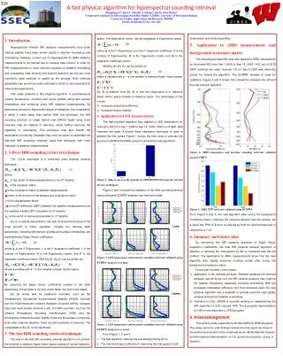
5. Radiative transfer approximation of single cloud layer model

6. Simulations performed • Nadir view, OD = 0, 0.1, 0.5, 1, 2, 3, 5 @ 10 um • Liquid clouds (Mie spheres, gamma dist.) • 1, 2, 3 km cloud top altitude • 2, 10, 20, 40 um Deff • Ice clouds (Hexagonal ice crystals, gamma dist.) • 5, 10, 15 km cloud top altitude • 10, 20, 40, 100 um Deff • Labels • “FAST” • Single-layer cloud fast radiative transfer model • “TRUTH” • LBLRTM/DISORT

7. What is “TRUTH” ? • The output of LBLDIS ! • gas layer optical depths from LBLRTM v6.01 • layers populated with particulate optical depths, assymetry parameters and single scattering albedos. • DISORT invoked to compute multiple scattered TOA radiances. • Radiances spectrally reduced to GIFTS channels and converted to brightness temperature.

8. LW band TRUTH brightness T spectrum

9. LW band difference spectra

10. Clear sky model bias removed

11. http://www.ssec.wisc.edu/gifts/noaa/

12. Surface emissivity effect on FAST model brightness temperatures Clear sky Liq. Cloud OD=5, De=10um @ 500 hPa Ice Cloud OD=5, De=30um @ 200 hPa

13. Two layer cloud model from Texas A&M coupled with UW/CIMSS clear-sky model 3 ice cloud models, 1 water cloud model 100-3246 1/cm (~3-100 um) Tropical De = 16-126 um Mid-latitude De = 8-145 um Polar De = 1.6-162 um Water-spheres De = 2-1100 um

14. Testing ly2g for idealised cases Altitude (km)

15. Clear-sky brightness temperature spectrum and surface emissivity for IGBP land class

16. Consistent cloud single scattering properties and hi-res RT model disort/g - asymmetry parameter disort/p - phase function @ 498 phase angles disort/p+s - plus solar source @ 30 deg zenith angle ly2g - LY2 executed for GIFTS channel bandpasses

17. Idealised cloud profile comparisons

18. Test atmospheric profiles from mesoscale model(s) MM5 simulation to provide more realistic test case cloudy profiles, this example at 4pm local time over U.S. mid-west.

19. 128 x 128 GIFTS cube of profiles over the Mid-west

20. netCDF GIFTS cubes and Unidata IDV

21. View from below

22. View from below

23. Realistic cloud profile comparisons - single layer/phase

24. Realistic cloud profile comparisons - two layer, thin cirrus 4

25. Realistic cloud profile comparisons - two layer, thick cirrus 2

26. Two-layer cloud formation model forLY2G • Automaticselection of multi-layer cloud type, height, visible optical depth, and effective diameter from MM5 cloud file for LY2G. • Multi-level clouds will be reorganized into two-layer cloud system from MM5 cloud file. • Layer cloud type, optical depth, and effective diameter will be estimated by weighting each • atmospheric level cloud properties in respect to mixing ratios of that level cloud particle habits. • Cloud top height is the level height of the uppermost level cloud in that layer. Layer cloud top Cloud layer Layer cloud bottom Atmosphere level Cloud layer Surface

27. Two-layer cloud formation model forLY2G (cont.) Automatic formation and selection of multi-layer cloud type, height, visible optical depth, and effective diameter from atmospheric profile for LY2G. Rationale: Cloud will be formed if the actual atmospheric relative humidity (RH) is equal to or greater than critical relative humidity (RHc) according to Dieter Klaes’s work (1984). where σ = P/Ps (P is atmospheric level pressure, and Ps is surface pressure.); α and β are two parameters controlling the value of the minimum of RHc and the height of the minimum. For the midlatitudes, if we use α =2 and β=, then RHc,min = 0.43 at a level σ = 0.65. The cloud phase or particle habit is simply a function of that level air temperature. Liquid/ice water mixing ratio MR is assumed being a fraction of water vapor saturation mixing ratio Ws. The ratio R=MR/Ws is generally determined by observation. Here R is assigned a value between 0.0002 – 0.0005, implying a supersaturation of 0.2% - 0.5%. Cloud particle effective diameter and visible optical depth will be estimated by cloud water/ice path calculated from water/ice mixing ratio and cloud thickness.

28. Two-layer cloud formation model forLY2G (cont.) MM5 Cloud file Atmosphere profile Two-layer cloud formation model has been incorporated into LY2G for the automatic two layer cloud system generation. Users still have option to manually input cloud information as they wish for code development and testing.

29. Current Status • We have implemented the two-layer cloud model in the framework of the GIFTS fast model (ly2g) and included access to an ecosystem surface emissivity model (MODIS band resolution) - less than 1s per GIFTS spectrum (3000+ chans). • We have created a system for generating ly2g and LBLRTM/DISORT (Dave Turner’s LBLDIS) simulated brightness temperatures for GIFTS channels and equivalent cloudy profiles. [Those computed by LBLDIS operate on a vertical profile of cloud properties, ly2g must select approximately equivalent thin layer height/OD/radii for up to two layers]. • We have automated the selection of cloud layer type, heights, ODs, effective radii from mesoscale model outputs, and atmosphere profiles (to be implemented). • We have added a netCDF interface option to make easier the visualization of inputs/outputs with Unidata’s IDV.

30. Further Work • LBLDIS is well suited to simulation of ground and aircraft observations but introduces some inaccuracies in simulating TOA brightness temperatures for any practical wavenumber step (up to 300 hPa, 0.01 cm-1 is fine; above 100 hPa even 0.001 cm-1 is inaccurate at the ~ 0.5 K level). The problem here is to provide the scattering code (required to simulate the underlying scattering/emitting atmosphere) with the angular distribution of the downwelling spectral radiance from the overlying emitting atmosphere - you can aggregate the upper level downwelling radiances to the scattering code spectral step size, and interpolate the lower level exitance to the smaller step size required for upper atmosphere RT. A coding task. • We need to address the inclusion of solar illumination in order to work confidently with the short wavelength end of the GIFTS spectrum. At high spectral resolution, variations in the solar spectrum itself can introduce further uncertainties. • Inclusion of a limited set of aerosol types - our collaborators at TAMU are already working on parameterizing their single scattering properties.

31. Finish (The End)