Download
1 / 18
180 likes | 397 Views
GIFTS-IOMI Clear Sky Forward Model Status Line-by-line Model Fast Model Future Plans Line-by-line Model Fast Model. Presented by David Tobin MURI Workshop, 27-28 May 2003, UW-Madison. Definition of terms:. Input parameters :. Forward (Radiance) model :.

E N D
GIFTS-IOMI Clear Sky Forward Model • Status • Line-by-line Model • Fast Model • Future Plans • Line-by-line Model • Fast Model Presented by David Tobin MURI Workshop, 27-28 May 2003, UW-Madison
Definition of terms: Input parameters : Forward (Radiance) model : Tangent Linear (TL) model : etc ... Adjoints (transpose of TL model) : Jacobian : • Monochromatic absorption and radiative transfer algorithms: • LBLRTM: Line-by-line Radiative Transfer Model • kCARTA: k Compressed Atmospheric Radiative Transfer Algorithm • Fast Model Approaches: • PLOD: Pressure Layer Optical Depth • OPTRAN: Optical Path Transmittance algorithm • OSS: Optimal Spectral Sampling
Water vapor absorption modeling H2O lines and continuum coefficients CKDv0 c-functions
GIFTS-IOMI Clear Sky Forward Model • Status • Line-by-line Model • Fast Model • Future Plans • Line-by-line Model • Fast Model
recent line-by-line development efforts. LBLRTM and kCARTA • ARM Site Atmospheric State Best Estimate products • The AERI / LBLRTM QME • longwave window water vapor continuum • MTCKD v1.0 continuum module • H2O • 15mm CO2 • AIRS obs-calcs • non-Local Thermodynamic Equilibrium • CO2 line-mixing at 4.3mm • upper level water channels and the water vapor continuum • 710-720 1/cm
AERI (downwelling at surface) obs-calc SGP ARM site, 22 July 2001, clear sky, LBLRTM
AIRS (upwelling at TOA) obs-calcs SGP ARM site, Sep ‘02 to Feb ‘03, night, ~clear sky, kCARTA (Dec ‘02 Delivery)
PLOD • current UW effort • Polychromatic regression based model with fixed pressure levels following UMBC approach, but currently with LBLRTM physics • Status: • “task0” is finished • Model is characterized, but performance is sub-par. Why ? • Regressions using SVDs and optical depth weighting • Incorporating kCARTA • Incorporating Adjoint and Tangent Linear modules • OPTRAN • NOAA effort • Polychromatic regression based model with fixed optical depth levels, currently with LBLRTM physics. Includes adjoint and tangent linear modules. • Status: • GIFTS spectral parameters provided to NOAA • model built for GIFTS will be available in a few months • OSS • AER, Inc. effort • New approach using linear combination of selected monochromatic frequencies to represent channel radiances. LBLRTM based. • A portion of the algorithm is patented. • Has advantages due to the use of real (monochromatic) transmittances. • Status: • gaining experience with a NASTI model • considering obtaining a model for GIFTS
------- GIFTS NeDT@296K ------- OSS RMS upper limit* Dependent Set Statistics: RMS(LBL-FM) heritage model MURI version MURI model w/ OD weighted SVD AIRS model c/o L. Strow, UMBC OSS model c/o Xu Liu, AER, Inc. OPTRAN, AIRS 281 channel set c/o PVD
------- GIFTS NeDT@296K Dependent Set Statistics: Mean(LBL-FM) heritage model MURI version MURI model w/ OD weighted SVD AIRS model c/o L. Strow, UMBC OSS model c/o Xu Liu, AER, Inc. OPTRAN, AIRS 281 channel set c/o PVD “negligible” “zero”
Spectral correlation (LBL-FM), GIFTS Model, SVD w/ OD weighting
GIFTS-IOMI Clear Sky Forward Model • Status • Line-by-line Model • Fast Model • Future Plans • Line-by-line Model • Fast Model
Line-by-Line Model. Future Plans • With the exception of a few spectral regions/issues, the line-by-line models kCARTA and LBLRTM are “converging” in general. Based on analysis of the highest quality validation cases, most spectral regions show absolute accuracy at or below the ~0.5 K level. • Remaining issues/efforts: • Produce a “ground-up” estimate of line-by-line model errors • Investigate temperature dependence of foreign broadened water vapor continuum • Evaluate uncertainty of upper level water vapor “truth”, and the nature of the 1400-1800 1/cm water vapor continuum and near wing lineshape • Intercompare LBLRTM and kCARTA approaches to CO2 15mm lineshape • Further validation of LBLRTM with upwelling TOA data (e.g. AIRS) and further validation of kCARTA with downwelling surface (e.g. AERI) data. • Evaluate need for non-LTE in GIFTS model • Investigate 710-720 1/cm obs-calcs
Biggest uncertainty wrt upper level water vapor forward model is knowledge and parameterization of the foreign broadened water vapor continuum component of the absorption (Cf0). For upper level water channels, the forward model is most certain at ~ 1587 1/cm, where a convergence of measurements and models of Cf0 exists. (CKDv2.4 is/was known to be in error in this region and has since been fixed.) “On-line” channels, which sense highest in the atmosphere, also have higher certainty because contribution from Cf0 is small for these channels.
Fast Model. Future Plans • UW PLOD model • Solve our accuracy problem • Finish Adjoint, TL, and jacobian modules • Re-make model with kCARTA and new dependent set profiles (UMBC 48 or UKMET 52) • Allow non-unit emissivity and add surface reflectance terms • Break-out other trace gases. CO, CH4, CO2, … • Obtain and gain experience with OPTRAN model from NOAA • Obtain OSS model from AER (?) • Evaluate PLOD vs. OPTRAN vs. OSS
The End Thank You