Motion and Optical Flow
300 likes | 335 Views
Motion and Optical Flow. Moving to Multiple Images. So far, we’ve looked at processing a single image Multiple images Multiple cameras at one time: stereo Single camera at many times: video (Multiple cameras at multiple times). Applications of Multiple Images. 2D Feature / object tracking

Motion and Optical Flow
E N D
Presentation Transcript
Moving to Multiple Images • So far, we’ve looked at processing asingle image • Multiple images • Multiple cameras at one time: stereo • Single camera at many times: video • (Multiple cameras at multiple times)
Applications of Multiple Images • 2D • Feature / object tracking • Segmentation based on motion • 3D • Shape extraction • Motion capture
Applications of Multiple Imagesin Graphics • Stitching images into panoramas • Automatic image morphing • Reconstruction of 3D models for rendering • Capturing articulated motion for animation
Applications of Multiple Imagesin Biological Systems • Shape inference • Peripheral sensitivity to motion • Looming field – obstacle avoidance • Very similar applications in robotics
Looming Field • Pure translation: motion looks like it originates at a point – focus of expansion
Key Problem • Main problem in most multiple-image methods: correspondence
Correspondence • Small displacements • Differential algorithms • Based on gradients in space and time • Dense correspondence estimates • Most common with video • Large displacements • Matching algorithms • Based on correlation or features • Sparse correspondence estimates • Most common with multiple cameras / stereo
Result of Correspondence • For points in image i displacements to corresponding locations in image j • In stereo, usually called disparity • In video, usually called motion field
Computing Motion Field • Basic idea: a small portion of the image(“local neighborhood”) shifts position • Assumptions • No / small changes in reflected light • No / small changes in scale • No occlusion or disocclusion • Neighborhood is correct size: aperture problem
Actual and Apparent Motion • If these assumptions violated, can still use the same methods – apparent motion • Result of algorithm is optical flow (vs. ideal motion field) • Most obvious effects: • Aperture problem: can only get motion perpendicular to edges • Errors near discontinuities (occlusions)
Computing Optical Flow:Preliminaries • Image sequence I(x,y,t) • Uniform discretization along x,y,t –“cube” of data • Differential framework: compute partial derivatives along x,y,t by convolving with derivative of Gaussian
Computing Optical Flow:Image Brightness Constancy • Basic idea: a small portion of the image(“local neighborhood”) shifts position • Brightness constancy assumption
Computing Optical Flow:Image Brightness Constancy • This does not say that the image remainsthe same brightness! • vs. : total vs. partial derivative • Use chain rule
Computing Optical Flow:Image Brightness Constancy • Given optical flow v(x,y) Image brightness constancy equation
Computing Optical Flow:Discretization • Look at some neighborhood N:
Computing Optical Flow:Least Squares • In general, overconstrained linear system • Solve by least squares
Computing Optical Flow:Stability • Has a solution unless C = ATA is singular
Computing Optical Flow:Stability • Where have we encountered C before? • Corner detector! • C is singular if intensity is constant or if there’s an edge • Use eigenvalues of C: • to evaluate stability of optical flow computation • to find good places to compute optical flow(finding good features to track)
Computing Optical Flow:Improvements • Assumption that optical flow is constant over neighborhood not always good • Decreasing size of neighborhood C more likely to be singular • Alternative: weighted least-squares • Points near center = higher weight • Still use larger neighborhood
Computing Optical Flow:Weighted Least Squares • Let W be a matrix of weights
Computing Optical Flow:Improvements • What if windows are still bigger? • Adjust motion model: no longer constant within a window • Popular choice: affine model
Computing Optical Flow:Affine Motion Model • Translational model • Affine model
Computing Optical Flow:Improvements • Larger motion: how to maintain “differential” approximation? • Solution: iterate • Even better: adjust window / smoothing • Early iterations: use larger Gaussians to allow more motion • Late iterations: use less blur to find exact solution, lock on to high-frequency detail
Computing Optical Flow:Lucas-Kanade • Iterative algorithm: • Set s = large (e.g. 3 pixels) • Set I’ I1 • Set v 0 • Repeat while SSD(I’, I2) > t • v += Optical flow(I’ I2) • I’ Warp(I1, v) • After n iterations,set s = small (e.g. 1.5 pixels)
Computing Optical Flow:Lucas-Kanade • I’ always holds warped version of I1 • Best estimate of I2 • Gradually reduce thresholds • Stop when difference between I’ and I2 small • Simplest difference metric = sum of squared differences (SSD) between pixels
Optical Flow Applications Video Frames [Feng & Perona]
Optical Flow Applications Optical Flow Depth Reconstruction [Feng & Perona]
Optical Flow Applications Obstacle Detection: Unbalanced Optical Flow Temizer
Optical Flow Applications • Collision avoidance: keep optical flow balanced between sides of image Temizer