Optical flow and Tracking
260 likes | 428 Views
Optical flow and Tracking. CISC 649/849 Spring 2009 University of Delaware. Outline. Fusionflow Joint Lucas Kanade Tracking Some practical issues in tracking. What smoothing to choose?. Stereo Matching results…. Difficulties in optical flow.

Optical flow and Tracking
E N D
Presentation Transcript
Optical flow and Tracking CISC 649/849 Spring 2009 University of Delaware
Outline • Fusionflow • Joint Lucas Kanade Tracking • Some practical issues in tracking
Difficulties in optical flow • Cannot directly apply belief propagation or graph cut • Number of labels too high • Brightness variation higher than stereo matching
Formulation as a labeling problem • Given flows x0 and x1, find a labeling y • Combine the flows to get a new flow xf
Proposal Solutions • Horn and Shunck with different smoothing • Lucas Kanade with different window sizes • Shifted versions of above
Discrete Optimization • Choose one of the proposals randomly as initial flow field • Visit other proposals in random order and update labeling • Combine the proposals according to the labeling to give fused estimate
Continuous Optimization • Some areas may have same solution in all proposals • Use conjugate gradient method on the energy function to decrease the energy further • Use bicubic interpolation to calculate gradient
denotes convolution with an integration • window of size ρ • differentiating with respect to u and v, setting • the derivatives to zero leads to a linear system: Recap… Lucas Kanade (sparse feature tracking) Horn Schunck (dense optic flow) • assumes unknown displacement u of a pixel is • constant within some neighborhood • i.e., finds displacement of a small window • centered around a pixel by minimizing: • regularizes the unconstrained optic flow equation • by imposing a global smoothness term • computes global displacement functions u(x, y) • v(x, y) by minimizing: • λ: regularization parameter, Ω: image domain • minimum of the functional is found by solving the • corresponding Euler-Lagrange equations, • leading to:
Limitations of Lucas-Kanade Tracking • Tracks only those features whose minimum eigenvalue is greater than a fixed threshold • Do edges satisfy this condition? • Are edges bad for tracking? • How can this be corrected?
Joint Lucas Kanade Tracking For each feature i, 1. Initialize ui ← (0, 0)T 2. Initialize i For pyramid level n − 1 to 0 step −1, 1. For each feature i, compute Zi 2. Repeat until convergence: (a) For each feature i, i. Determine ii. Compute the difference It between the first image and the shifted second image: It (x, y) = I1(x, y) − I2(x + ui , y + vi) iii. Compute ei iv. Solve Ziu′i = ei for incremental motion u’i v. Add incremental motion to overall estimate: ui ← ui + u′i 3. Expand to the next level: ui ← aui, where a is the pyramid scale factor
How to find mean flow? • Average of neighboring features? • Too much variation in the flow vectors even if the motion is rigid • Calculate an affine motion model with neighboring features weighted according to their distance from tracked feature
What features to track? Given the Eigen values of a window are emax and emin • Standard Lucas Kanade chooses windows with emin > Threshold • This restricts the features to corners • Joint Lucas Kanade chooses windows with max(emin,K emax ) > Threshold where K<1.
Results LK JLK
Observations • JLK performs better on edges and untextured regions • Aperture problem is overcome on edges • Future improvements • Does not handle occlusions • Does not account for motion discontinuities
Some issues in tracking • Appearance change • Sub pixel accuracy • Lost Features/Occlusion
Further reading • Joint Tracking of Features and Edges. Stanley T. Birchfield and Shrinivas J. Pundlik. CVPR 2008 • FusionFlow: Discrete-Continuous Optimization for Optical Flow Estimation. V. Lempitsky, S. Roth, C. Rother. CVPR 2008 • The template update problem, Matthews, L.; Ishikawa, T.; Baker, S. PAMI 2004