Multiple Regression
Advanced Quantitative Methods in Comparative Social Sciences http://statisticalmethods.wordpress.com. Multiple Regression. In reality data are scattered. For z scores. Correlation - measures the size & the direction of the linear relation btw. 2 variables (i.e. measure of association)

Multiple Regression
E N D
Presentation Transcript
Advanced Quantitative Methods in Comparative Social Scienceshttp://statisticalmethods.wordpress.com Multiple Regression
Correlation - measures the size & the direction of the linear relation btw. 2 variables (i.e. measure of association) - unitless statistic (it is standardized); we can directly compare the strength of correlations for various pairs of variables The stronger the relationship between X & Y, the closer the data points will be to the line; the weaker the relationship, the farther the data points will drift away from the line. Pearson’s r = the sum of the products of the deviations from each mean, divided by the square root of the product of the sum of squares for each variable. If X and Y are expressed in standrad scores (i.e. z-scores), we have Z(y) = β*Z(x)and r = Σ(Zy*Zx)/N = beta
The Multiple Regression Model Ŷ = a + b1X1 + b2X2 + ... + biXi - this equationrepresents the best prediction of a DV from several continuous (or dummy) IVs; i.e. itminimizes the squared differences btw. Y and Ŷ least square regression Goal: arrive at a set of regression coefficients (bs) for the IVs that bring Ŷs as close as possible to Ys values Regression coefficients: minimize (the sum of squared) deviations between Ŷ and Y; optimize the correlation btw. Ŷ and Y for the data set.
Three criteria for a number of independent (exploratory) variables: (1) Theory (2) Parsimony (3) Sample size
Common Research Questions • Is the multiple correlation between the DV and the IVs statistically significant? • If yes, which IVs in the equation are important, and which not? • Does adding a new IV to the equation improve the prediction of the DV? • Is prediction of a DV from one set of IVs better than prediction from another set of IVs? Multivariate regression also allows for non-linear relationships, by redefining the IV(s): squaring, cubing, .. of the original IV
Assumptions • Random sampling; • DV = continuous; IV(s) variables = continuous (can be treated as such), or dummies; • Linear relationship btw. the DV& the IVs variables (but we canmodel non-linear relations); • Normally distributed characteristics of Y in the population; • Normality, linearity, and homoskedasticity btw. predicted DV scores (Ŷs) and the errors of prediction (residuals) • Independence of errors; • No large outliers
Initial checks 1. Cases-to-IVs Ratio Rule of thumb: N>= 50 + 8*m for testing the multiple correlation; N>=104 + m for testing individual predictors, where m = no. of IVs Need higher case-to-IVs ratio when: • the DV is skewed (and we do not transform it); • a small effect size is anticipated; • substantial measurement error is to be expected 2. Screening for outliers among the DV and the IVs 3. Multicollinearity - too highly correlated IVs are put in the same regression model
4.Assumptions of normality, linearity, and homoskedasticity btw. predicted DV scores (Ŷs) and the errors of prediction (residuals) 4.a. Multivariate Normality • each variable & all linear combinations of the variables are normally distributed; • if this assumption is met residuals of analysis = normally distributed & independent For grouped data: assumption pertains to the sampling distribution of means of variables; Central Limit Theory: with sufficiently large sample size, sampling distributions are normally distributed regardless of the distribution of the variables What to look for (in ungrouped data): • is each variable normally distributed? Shape of distribution: skewness & kurtosis. Frequency histograms; expected normal probability plots; detrend expected normal probability plots • are the realtionships btw. pairs of variables (a) linear, and (b) homoskedastic (i.e. the variance of one variable is the same at all values of other variables)?
Homoskedasticity • for ungrouped data: the variability in scores for one continuous variable is ~ the same at all values of another continuous variable • for grouped data: the variability in the DV is expected to be ~ the same at all levels of the grouping variable Heteroskedasticity = caused by: • non-normality of one of the variables; • one variable is related to some transformation of the other; • greater error of measurement at some level of an IV
Residuals Scatter Plots to check if: 4.a. Errors of prediction are normally distributed around each & every Ŷ 4.b. Residuals have straight line relationship with Ŷs - If genuine curvilinear relation btw. an IV and the DV, include a square of the IV in the model 4.c. The variance of the residuals about Ŷs is ~the same for all predicted scores (assumption of homoskedasticity) - heteroskedasticity may occur when: - some of the variables are skewed, and others are not; may consider transforming the variable(s) - one IV interacts with another variable that is not part of the equation 5. Errors of prediction are independent of one another Durbin-Watson statistic = measure of autocorrelation of errors over the sequence of cases; if significant it indicates non-independence of errors

