Download

1 / 32
350 likes | 704 Views
V Completely Randomized Factorial Design A. Characteristics of a CRF- pq Design 1. Design has two treatments denoted by A and B . Treatment A has j = 1, . . . , p levels; treatment B has k = 1, . . . , q levels.

E N D
V Completely Randomized Factorial Design A. Characteristics of a CRF-pq Design 1. Design has two treatments denoted by A and B. Treatment A has j = 1, . . . , p levels; treatment B has k = 1, . . . , q levels. 2. Each level of treatment A appears once with each level of treatment B, and vice versa.
3. N participants are randomly assigned to the pq treatment combinations with n in each combination. B. Sample Model Equation for Participant i in Treatment Combination aj and bk.
C. Partition of the Total Sum of Squares (SSTO) 1. The total variability among scores is a composite that can be decomposed into treatment A sum of squares (SSA)
treatment B sum of squares (SSB) interaction sum of squares (SSAB) within cell sum of squares (SSWCELL)
D. Degrees of Freedom for SSTO, SSA, SSB, SSAB, and SSWCELL 1. dfTO = npq – 1 2. dfA = p – 1 3. dfB = q – 1 4. dfAB = (p – 1)(q – 1) 5. dfWCELL = pq(n – 1)
E. Mean Squares and F Statistic 1. SSTO/(npq – 1) = MSTO 2. SSA/(p – 1) = MSA 3. SSB/(q – 1) = MSB 4. SSAB/(p – 1)(p – 1) = MSAB 5. SSWCELL/pq(n – 1) = MSWCELL
VI Computational Procedures for a CRF-23 Design A. Descriptive Statistics for Reading-Speed Data 1. Treatment A: a1 = 15 ft-c of illumination a2 = 30 ft-c of illumination 2. Treatment B: b1 = 6-pt type b2 = 12-pt type b3 = 18-pt type
Table 3. Descriptive Summary of Reading-Speed Data Illumination Type Size Level b1 = 6-pt b2 = 12-pt b2 = 18-pt 382 423 436 a1 = 15 ft-c 413.7 35.1 28.2 29.1 26.2 423 442 441 a2 = 30 ft-c 435.3 27.8 28.4 29.6 27.0 402.5 432.5 438.5 34.3 29.4 25.2
Table 4. Computational Procedures for CR-23 Design ABS Summary Table a1 a1 a1 a2` a2 a2 b1 b1 b2 b2 b3 b3 378 454 432 415 439 426 408 394 411 396 467 428 357 452 466 451 477 464 353 396 411 455 410 412 414 419 460 398 417 475 1910 2115 2180 2115 2210 2205
Table 4. (continued) AB Summary Table b1 b2 b3 a1 1910 2115 2180 6205 a2 2115 2210 2205 6530 4025 4325 4385
Table 4. (continued) SSTO = [ABS] – [X] = 5,437,581.000 – 5,406,007.500 = 31,573.500 SSA = [A] – [X] = 5,409,528.333 – 54,06,007.500 = 3,520.833 SSB = [B] – [X] = 5,413,447.500 – 5,406,007.500 = 7,440.000 SSAB = [AB] – [A] – [B] + [X] = 5,418,615.000 – 5,409,528.333 – 413,447.500 + 5,406,007.500 = 1,646.667 SSWCELL = [ABS] – [AB] = 5,437,581.000 – 5,418,615.000 = 18,966.000
Table 5. ANOVA Table for CRF-23 Design Source SS df MS F 1. Treatment A 3520.833 p – 1 = 1 3520.833 4.46* (illumination level) 2. Treatment B 7440.000 q – 1 = 2 3720.000 4.718 (size of type) 3. AB interaction 1646.667 (p – 1)(q – 1) = 2 823.334 1.04 4. Within Cell 18966.000 pq(n – 1) = 24 790.250 5. Total 31573.500 npq – 1 = 29 *p < .05
B. Interpretation of Interactions Figure 3. Graph of the nonsignificant AB interaction
Figure 4. When the AB interaction is significant, the interpretation of treatment A and treatment B is misleading.
Figure 5. A significant interaction does not mean that all lines throughout their length are nonparallel. A significant interaction does mean that there are at least two nonparallel lines between at least two levels of the other treatment.
C. Assumptions for CRF-pq Design 1. The model equation reflects all of the sources of variation that affect Xijk. 2. Participants are random samples from the respective populations or the participants have been randomly assigned to the treatment combinations.
3. The population for each of the pq treatment combinations is normally distributed. 4. The variances of each of the pq treatment combinations are equal.
VII Multiple Comparisons A. Fisher-Hayter Test Statistic 1. Treatment A Critical value for the Fisher-Hayter statistic is q; p – 1, , where = pq(n – 1).
2. Treatment B Critical value for the Fisher-Hayter statistic is q; q – 1, = q.05; 3 – 1, 24 = 2.92, where = pq(n – 1) = 24.
B. Scheffé Test Statistic 1. Treatment A Critical value for Scheffé’s statistic is (p – 1)F; 1, 2, where = p – 1 and = pq(n – 1).
2. Treatment B Critical value for Scheffé’s statistic is (q – 1) F;1,2, where = q – 1 and = pq(n – 1).
C. Scheffé Two-Sided Confidence Interval 1. Treatment A
VIII Practical Significance A. Partial Omega Squared 1. Treatment A, ignoring treatment B and the AB interaction 2. Computation for type size, treatment A
3. Treatment B, ignoring treatment A and the AB interaction 4. Computation for room illumination, treatment B
4. AB interaction, ignoring treatments A and B 5. Computation for the AB interaction
B. Hedges’s g Statistic 1. Treatment A