Factorial ANOVA
Factorial ANOVA. Cal State Northridge 320 Andrew Ainsworth PhD. Topics in Factorial Designs. What is Factorial? Assumptions Analysis Multiple Comparisons Main Effects Simple Effects Simple Comparisons Effect Size estimates Higher Order Analyses. Factorial?. Factorial – means that:

Factorial ANOVA
E N D
Presentation Transcript
Factorial ANOVA Cal State Northridge 320 Andrew Ainsworth PhD
Topics in Factorial Designs • What is Factorial? • Assumptions • Analysis • Multiple Comparisons • Main Effects • Simple Effects • Simple Comparisons • Effect Size estimates • Higher Order Analyses Psy 320 - Cal State Northridge
Factorial? • Factorial – means that: • You have at least 2 IVs • And all levels of one variable occur in combination with all levels of the other variable(s). • Assumptions • Same as one-way ANOVA but they are tested within each cell • i.e. Normality, Homogeneity and Independence Psy 320 - Cal State Northridge
Simplest Form: 2 x 2 ANOVA Psy 320 - Cal State Northridge
Analysis • Performing a factorial analysis does the job of three analyses in one • Two one-way ANOVAs, one for each IV (called a main effect) • And a test of the interaction between the IVs • Interaction? – the effect of one IV depends on the level of another IV • The variability that is left over after you assess each IV • The 2 IVs together work to affect scores over and above either of them independently Psy 320 - Cal State Northridge
Analysis • The between groups sums of squares from 1-way ANOVA is further broken down: • Before SSbg = SSeffect • Now SSbg = SSA + SSB + SSAB • In a two IV factorial design A, B and AxB all differentiate between groups, therefore they all add to the SSbg Psy 320 - Cal State Northridge
Analysis • Total variability = (variability of A around GM) + (variability of B around GM) + (variability of each group mean {AB} around GM) + (variability of each person’s score around their group mean) • SSTotal = SSA + SSB + SSAB + SSerror Psy 320 - Cal State Northridge
Analysis • Degrees of Freedom • dfA = #groupsA – 1 • dfB = #groupsB – 1 • dfAB = (a – 1)(b – 1) • dferror= ab(n – 1) = abn – ab = N – ab • dftotal = N – 1 = a – 1 + b – 1 + (a – 1)(b – 1) + N – ab Psy 320 - Cal State Northridge
Analysis • Breakdown of degrees of freedom • Breakdown of sums of squares Psy 320 - Cal State Northridge
Analysis • Mean square • The mean squares are calculated the same • SS/df = MS • You just have more of them, MSA, MSB, MSAB, and MSWG • This expands when you have more IVs • One for each main effect, one for each interaction (two-way, three-way, etc.) Psy 320 - Cal State Northridge
Analysis • F-test • Each effect and interaction is a separate F-test • Calculated the same way: MSeffect/MSWG since MSWG is our error variance estimate • You look up a separate Fcrit for each test using the dfeffect, dfWG and tabled values Psy 320 - Cal State Northridge
Example Psy 320 - Cal State Northridge
Sample data reconfigured into cell and marginal means (with variances) Analysis Psy 320 - Cal State Northridge
Example – Sums of Squares Psy 320 - Cal State Northridge
Example – Sums of Squares Psy 320 - Cal State Northridge
Example – Sums of Squares Psy 320 - Cal State Northridge
Example – Sums of Squares Psy 320 - Cal State Northridge
Example – Sums of Squares Psy 320 - Cal State Northridge
Analysis – Computational • Marginal Totals – we look in the margins of a data set when computing main effects • Cell totals – we look at the cell totals when computing interactions • In order to use the computational formulas we need to compute both marginal and cell totals Psy 320 - Cal State Northridge
Sample data reconfigured into cell and marginal totals Analysis – Computational Psy 320 - Cal State Northridge
Analysis – Computational • Formulas for SS
Analysis – Computational • Example Psy 320 - Cal State Northridge
Analysis – Computational • Example Psy 320 - Cal State Northridge
Analysis – Computational • Example Psy 320 - Cal State Northridge
Analysis – Computational • Example Psy 320 - Cal State Northridge
Analysis • Example • The MSWG is also the pooled (average) variance across the cells, since all n are equal: (.333+2.333+2.333+1+1+.333+2.333+0+.333)/9 = 1.111 Psy 320 - Cal State Northridge
Analysis • Fcrit(2,18)=3.55 • Fcrit(4,18)=2.93 • Since 15.25 > 3.55, the effect for profession is significant • Since 14.55 > 3.55, the effect for length is significant • Since 23.46 > 2.93, the effect for profession * length is significant Psy 320 - Cal State Northridge
Effect Size Revisited • Eta Squared is calculated for each effect • Omega Squared also for each effect Psy 320 - Cal State Northridge
Effect Size Example • Effect Size for Profession Psy 320 - Cal State Northridge
Multiple Comparisons • If a main effect is significant and has more than 2 levels, than you need to do marginal comparisons • If the interaction is significant • You should break the interaction down by performing a simple effect analysis of A at each level of B (The effect of A at B1, A at B2, A at B3, etc.) and vice versa • If any of them are significant and if A has more than 2 levels, follow up with simple comparisons Psy 320 - Cal State Northridge
Multiple Comparisons Psy 320 - Cal State Northridge
Specific Comparisons • If the comparisons were planned than analyze them without any adjustment to the critical value • If they were post-hoc than the values needs to be adjusted (e.g. Tukey, Bonferroni, etc.) • This is the same as previously covered Psy 320 - Cal State Northridge
Multiple Comparisons ExampleMain Effect: Profession Psy 320 - Cal State Northridge
Multiple Comparisons ExampleMain Effect: Length of Stay Psy 320 - Cal State Northridge
Higher-Order Designs • Higher-order – meaning more than 2 IVs • With 3 IVs; each with 2 levels you have a 2 x 2 x 2 design • If we have even 5 subjects per cell we are talking about a minimum of 40 subjects • We are also talking about: • SST = SSA + SSB + SSC + SSAB + SSAC + SSBC + SSABC + SSWG Psy 320 - Cal State Northridge
Higher-Order Designs • Higher-order – meaning more than 2 IVs • With 4 IVs; each with 2 levels you have a 2 x 2 x 2 x 2 design • If we have even 5 subjects per cell we are talking about a minimum of 80 subjects • We are also talking about: • SST = SSA + SSB + SSC + SSD + SSAB + SSAC + SSAD + SSBC + SSBD + SSCD + SSABC + SSABD + SSACD + SSBCD + SSABCD + SSWG Psy 320 - Cal State Northridge