Wave-Equation Migration in Anisotropic Media
450 likes | 714 Views
Wave-Equation Migration in Anisotropic Media. Jianhua Yu. University of Utah. Contents. Motivation. Anisotropic Wave-Equation Migration. Numerical Examples:. Cusp model. 2-D SEG/EAGE model. 3-D SEG/EAGE model. Conclusions. Contents. Motivation. Anisotropic Wave-Equation Migration.

Wave-Equation Migration in Anisotropic Media
E N D
Presentation Transcript
Wave-Equation Migration in Anisotropic Media Jianhua Yu University of Utah
Contents Motivation Anisotropic Wave-Equation Migration Numerical Examples: Cusp model 2-D SEG/EAGE model 3-D SEG/EAGE model Conclusions
Contents Motivation Anisotropic Wave-Equation Migration Numerical Examples: Cusp model 2-D SEG/EAGE model 3-D SEG/EAGE model Conclusions
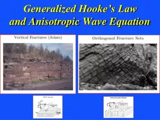
Irregular acquisition geometry Bandwidth source wavelet Velocity errors Higher order phenomenon: Anisotropy What Blurs Seismic Images?
Anisotropic wave-equation migration: Anisotropic Imaging Ray-based anisotropic migration: Anisotropic velocity model ---Ristow et al, 1998 ---Han et al. 2003
>78 wave propagator High efficiency Improve image accuracy o Develop 3-D anisotropic wave-equation migration method in orthorhombic model Objective:
Contents Motivation Anisotropy Wave-Equation Migration Numerical Examples: Cusp model 2-D SEG/EAGE model 3-D SEG/EAGE model Conclusions
General Wave Equation Wave equation in displacement Ui : displacement component Cijkl : 4th-order stiffness tensor
Eigensystem Equation Polarization components of P-P, SV, and SH waves
and Decoupled P plane Wave Motion Equations in (x,z) and (y,z) planes
det and det Decoupled P plane Wave Motion Equations in (x,z) and (y,z) planes
(y,z) plane Thomsen’s Parameters Dispersion Equations (x,z) plane
VTI: FFD algorithm
Velocity: Anisotropy: How to Set Velocity and Anisotropy Parameters a& b : Optimization coefficients of Pade approximation for FD
Pade Approximation Comparison 5 Error % 0 0 Angle 90
Pade Approximation Comparison 0.05 Beyond 78 within 0.02 % Error % 0 0 Angle 78
Contents Motivation Anisotropy Wave-Equation Migration Numerical Examples: Cusp model 2-D SEG/EAGE model 3-D SEG/EAGE model Conclusions
Exact Exact Approximation Approximation ** ** Strong Anisotropy Weak Anisotropy 0.6 Kz 0 -0.3 0.3 -0.3 0.3 Kx Kx
Dispersion Equation Approximation 0.3 Kz Strong anisotropy 0 -0.3 Kx 0.3
0 New V/V0=3 iso Depth (km) Standard V/V0=3 iso 2.0
V/V0=3 V/V0=3 0 Strong Aniso Depth (km) Weak Aniso 2.0
Contents Motivation Anisotropy Wave-Equation Migration Numerical Examples: Cusp model 2-D SEG/EAGE model 3-D SEG/EAGE model Conclusions
Velocity (2.0-3.0 km/s) X (km) 0 1.5 0 Depth (km) 1
Velocity (2.0-3.0 km/s) Isotropic data (SUSYNLY) Anisotropic data (SUSYNLVFTI) X (km) X (km) 0 1.5 0 1.5 0 0 Time (s) Time (s) 1.2 1
0 1.5 0 1.5 Anisotropic data Isotropic mig Anisotropic data Anisotropic mig X (km) 0 1.5 0 Depth (km) 1 Isotropic data Isotropic mig (su)
Contents Motivation Anisotropy Wave-Equation Migration Numerical Examples: Cusp model 2-D SEG/EAGE model 3-D SEG/EAGE model Conclusions
X (km) 0 5 0 Depth (km) Salt Model (VTI) 4
X (km) 0 5 0 Depth (km) 4 Iso-mig
X (km) 0 5 0 Depth (km) 4 VTI Aniso-mig
0 0 0 1.5 1.5 1.5 X (km) X (km) Anisotropy Error 20 % Anisotropy Error 40 % Inaccurate Thomsen’s Parameters (VTI) X (km) 0 Depth (km) 4 Anisotropy Error 10 %
Inaccurate Thomsen’s Parameters 5 10 X (km) X (km) X (km) 5 10 5 10 3 Depth (km) 4 Anisotropy Error 10 % Anisotropy Error 20 % Anisotropy Error 40 %
Contents Motivation Anisotropy Wave-Equation Migration Numerical Examples: Cusp model 2-D SEG/EAGE VTI model 3-D SEG/EAGE VTI model Conclusions
X (km) 0 5 Iso (y=1.5 km) X (km) 0 5 0 Depth (km) 4 VTI Aniso (y=1.5 km)
Y (km) 0 5 Iso (x=1.5 km) Y (km) 0 5 0 Depth (km) VTI Aniso (x=1.5 km) 4
Y (km) 0 5 Y (km) 0 5 0 Depth (km) Iso (x=3 km) VTI Aniso (x=3 km) 4
Iso (z=0.5 km) X (km) X (km) 0 5 0 5 0 VTI Aniso (z=0.5 km) Y (km) 5
Iso (z=2.5 km) X (km) X (km) 0 5 0 5 0 VTI Aniso (z=2.5 km) Y (km) 5
Contents Motivation Anisotropy Wave-Equation Migration Numerical Examples: Cusp model 2-D SEG/EAGE model 3-D SEG/EAGE model Conclusions
Works for 2-D and 3-D media Valid for VTI and TI Improves spatial resolution o • 78 Propagator Cost = Cost of Standard 45^o propagator Conclusions o New > 78 Anisotropic wave propagator:
Thanks To 2003 UTAM Sponsors CHPC