Download
1 / 24
240 likes | 495 Views
4. Atmospheric chemical transport models. 4.1 Introduction 4.2 Box model 4.3 Three dimensional atmospheric chemical transport model. 4.1 Introduction. Questions What is the contribution of source A to the concentration of pollutants at site B?

E N D
4. Atmospheric chemical transport models 4.1 Introduction 4.2 Box model 4.3 Three dimensional atmospheric chemical transport model
4.1 Introduction Questions • What is the contribution of source A to the concentration of pollutants at site B? • What is the most cost-effective strategy for reducing pollutant concentrations below an air quality standard? • What will be the effect on air quality of the addition of the reduction of a specific air pollutant emission flux? • What should one place a future source to minimize its environmental impacts? • What will be the air quality tomorrow or the day after?
The atmosphere is an extremely reactive system in which numerous physical and chemical processes occur simultaneously. Mathematical models provide the necessary framework for integration of our understanding of individual atmospheric processes and study of their interaction. Three basic components of an atmospheric model are species emission, transport and physiochemical transformations
①Eulerian model: describes the concentrations in an array of fixed computational cells ②Lagrangian model: simulates concentration change of air parcel as it is advected in the atmosphere. 출처: http://www.romair.eu/model-description.php?l ang=en 출처: http://www.shodor.org/os411/courses/411f/module03/unit05/ page01.html
Classification based on dimension ① box model(상자 모델): zero-dimensional Concentrations are functions of time only. C(t) ② column model: one-dimensional Horizontally homogeneous layers Concentrations are functions of height and time. C(z, t) ③ two dimensional model: often used in description of global atmospheric chemistry ④ three dimensional model: c(x,y,z,t)
4.2 Box model (상자모델) 4.1.1 Eulerian box model Assume that the height (H) of the box equal the mixing layer height. : background concentration : mass emission rate kg/h-1 : chemical production rate (kg m-3 h-1) : removal rate(dry deposition, wet deposition)
1) For constant mixing height residence time
Problem 1 Ex1) An inert species has as initial concentration and is emitted at a rate . Assuming that its background concentration is , calculate its steady-state concentration over a city characterized by an average wind speed of 3m/s. Assume that the city has dimensions and a constant mixing height of 1000m.
2) For changing mixing height with time ① For decreasing mixing height No direct change of the concentration inside the mixed layer Because the box will be smaller, surface sources and sinks will have a more significant effect. ② For increasing mixing height Entrainment and subsequent dilution will change the concentration. : the concentration above the box.
Mass balance Neglecting
4.1.2 Lagrangian Box model • No advection term
Problem 2 Ex 2) SO2 is emitted in an urban area with a flux of 2000 g m-3. The mixing height over the area is 1000m, the atmospheric residence time 20h, and SO2reacts with an average rate of 3 % h-1. Rural areas around the city are characterized by a SO2 concentration equal to 2 g m-3 . What is the average SO2 concentration in the urban airshed for the above conditions? Assume an SO2 dry deposition velocity of 1cms-1and a cloud/ fog-free atmosphere
4.3 Three dimensional atmospheric chemical model : eddy diffusivity : emission rate : removal flux : Reactionrate Input data: three dimensional meteorological field, emission data, initial and boundary condition of pollutants Example of three dimensional model RADM(Regional Acid Deposition Model) UAM(Urban Airshed Model), CMAQ (Community Multiscale air quality) Chemical transport model
4.2.1 Coordinate system Terrain following coordinates
4.2.2 Initial conditions Start atmospheric simulations some period of time. At the end of start up period the model should have established concentration fields that do not seriously reflect the initial conditions. 4.2.3 Boundary condition Side boundary condition a function of time.
Unlike initial condition, boundary conditions, especially at the upwind boundaries, continue to affect predictions throughout the simulations. • Therefore, one should try to place the limits of the modeling domain in relatively clean areas where boundary conditions are relatively well know and have a relatively small effect on model predictions. • Uncertainty of side boundary conditions in urban air pollution model prediction may be reduced by use of larger scale models to provide the boundary condition to the urban scale model. : nesting technique
Upper boundary condition • Total reflection condition at the upper boundary of the computation domain • Alternative boundary condition (Reynolds et al., 1973) • for • for • : the concentration above the modeling region.
Lower boundary condition : deposition velocity of species : ground-level emission rate of the species.
4.2.4 Numerical solution of chemical transport models • A: Adevection operator • D: Diffusion operator • C: cloud operator • G: Gas-phase chemistry operator • P : Aerosol operator • S: source/sink operator
Operator splitting • Instead of solving the full equation at once, basic idea is to solve independently the pieces of the problem corresponding to the various processes and then couple the various changes resulting from the separate partial calculations.
The other alternatives • Order of operator application is another issue. • McRae et al. (1982a) T: transport operator : advection and diffusion
Diffusion Crank-Nicholson algorithm
Advection • : upwind finite difference scheme • : stable