Download
1 / 26
260 likes | 449 Views
Current AASPI Software Inventory (January 23, 2008). Computational requirements: A modern Fortran 90 compiler A recent SunOS or Linux operating system Willingness to install SEP utilities (software uses Stanford Exploration Project I/Oand graphics)

E N D
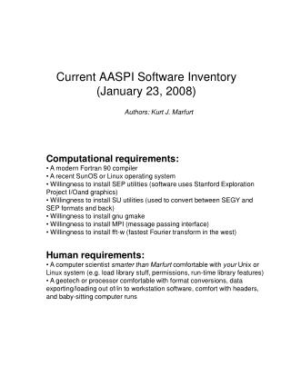
Current AASPI Software Inventory(January 23, 2008) • Computational requirements: • A modern Fortran 90 compiler • A recent SunOS or Linux operating system • Willingness to install SEP utilities (software uses Stanford Exploration Project I/Oand graphics) • Willingness to install SU utilities (used to convert between SEGY and SEP formats and back) • Willingness to install gnu gmake • Willingness to install MPI (message passing interface) • Willingness to install fft-w (fastest Fourier transform in the west) Authors: Kurt J. Marfurt • Human requirements: • A computer scientist smarter than Marfurt comfortable with your Unix or Linux system (e.g. load library stuff, permissions, run-time library features) • A geotech or processor comfortable with format conversions, data exporting/loading out of/in to workstation software, comfort with headers, and baby-sitting computer runs
AASPI Attribute Software Inventory • Basic geometric attributes (all performed with analytic trace) (program geom_attr) • Dip and azimuth • Total energy and coherent energy within a window • Confidence measure within a window • Energy-weighted coherent amplitude gradients: • Fractional derivative of amplitude: • Three edge algorithms: • coherent_energy/total_energy • outer product of covariance matrix: • correlation between d and dH • Measures of reflector shape and 2nd derivatives of amplitude (program reflector_shape) • Most negative and most positive curvature • Maximum and minimum curvature • Azimuth of minimum curvature • Gaussian and mean curvature • Reflector rotation (non quadratic surface) • Shape index and curvedness • Dome, ridge, saddle, valley, and bowl shape ‘components’ • Lineaments (i.e. amplitude of ridges and valleys) • Lineament count for subsequent rose diagrams • Crude estimate of reflector divergence/convergence • Crude estimate of angular unconformities • Azimuth-limited lineament volumes
AASPI Attribute Software Inventory • Edge-preserving, structure-oriented filtering (program geom_attr) • mean • median • principle component (also called Kohonen-Loeve filter) • Spectral decomposition (program spec_cmp) • wavelet time, frequency, phase, and envelope • spectral amplitude and phase components at each frequency • spectral balancing • amplitude, amplitude above spectral average, frequency and phase of spectral peak • reconstructed wavefield (with or without spectral balancing) • Composite display utilities (programs hl_plot, hl_gray_plot,…) • 2-D color bars (e.g. hue vs lightness or hue vs. saturation) • 3-D color bars (e.g. hue vs. lightness vs. saturation) • Boolean composite images (a type of overplot) • Rose diagrams (programs generate_roses, and display_roses) • roses stenciled onto SEGY format volumes? • Volumetric image processing (program image_filter) • mean, median, and alpha-trim mean filters • confidence-weighted mean, median, and alpha-trim mean filters • dip oriented image processing filters
35 Gbyte job – 16 hrs on 46 2.5GHz processor (output 8 volumes) (cost of hardware ~ $100,000 US) Loading each volume into Geoframe – 4 hrs Slicing each volume inside Geoframe – 8 hrs Ratio of loading and slicing to compute time : 6
Seismic data Read seismic data Send overlapping data blocks to slaves Seismic data on slave Seismic data on slave Seismic data on slave Seismic data on slave
Seismic data on slave Compute dip components in window centered about each node Assign dip to be that of overlapping window having the most coherent data in most coherent window in centered window Calculate mean amplitude along dip Calculate KL filtered data along dip Project vectors against covariance matrix Calculate amplitude gradients Calculate median amplitude along dip Calculate coherent and total energy Send results to master Send results to master Send results to master Send results to master Send results to master Send results to master Send results to master Write output to disk Collect blocks of output
Curv neg Coh 1.0 0 pos 0.8 R R R’ Q Q Q P P P’ P P P R R R Q Q Q (a) (b) (c) Figure 1. Attribute expression of reverse faulting, giving rise to strike slip faulting and pop-up blocks - Teapot Dome, WY, USA. Horizon slices along the purple horizon shown in Figure 2 through (a) coherence, (b) most positive curvature, and (c) most negative curvature volumes. (After Chopra and Marfurt, 2006; Seismic data courtesy of RMOTC).
0.5 0.5 1.0 1.0 Time (s) Time (s) 1.5 1.5 (a) (b) Q Q P P R R (c) Figure 2. Seismic cross sections through faults seen in the curvature volumes in Figure 1: (a) dip line PP’, (b) strike line QQ’, and (c) a third line perpendicular to the curvature lineaments, RR’. The strike-slip fault indicated by the white arrows is a distinct discontinuity at this level, and therefore is seen in the coherence slice. The more subtle faults indicated by black arrows are not seen on the coherence, but are seen on the curvature horizon slices. (After Chopra and Marfurt, 2006; Seismic data courtesy of RMOTC).
A A B B C C (b) (a) A B C A B C A A B B C C A B C A B C (d) (c) 1 km A A B B C C 1.3 1.4 Time (s) 1.5 (g) (f) (e) Figure 3. Four views of a Winnepegosas reef from a survey acquired in Alberta, Canada: (a) EW and (b) NS components of the energy-weighted coherent amplitude gradient, (c) coherence, and (d) peak spectral frequency modulated by peak amplitude above average. Time slice at 1.438 s. Vertical slices through the seismic data along lines (e) AA’, (f) BB’, and (g) CC’. The 2-D color bar for peak frequency vs. amplitude of peak frequency is identical to the color bar in Figure 6. (After Chopra and Marfurt, 2006; Seismic data courtesy of Talisman).
4 km Peak frequency (Hz) 10 80 high N Amp above average A A A A low (b) (a) A A Coh 1.2 high 1.3 Time (s) 1.4 (d) A A 1.5 low (c) A A (e) (f) Figure 4. Time slices at 1.3 s showing multiple channels through (a) seismic data, (b) coherence, and (c) fractional derivative of amplitude volumes for a survey acquired in the South Marsh Island area, Gulf of Mexico, USA. (d) Vertical section through the seismic data along line AA’. White arrows indicate the two prominent channels seen in the time slice. Grey arrow indicates a fault. (e) Peak spectral frequency displayed against amplitude above average spectrum. (After Chopra and Marfurt, 2006; Seismic data courtesy of Fairfield).
4 km Curv N neg A A A A 0 pos (b) (a) Figure 5. Time slices at 1.3 s corresponding to those shown in Figure 4 through (a) most positive and (b) most negative structural curvature volumes. While the two intersecting faults show up well on the most negative curvature time slice, there is little indication of the channels that are so obvious on the amplitude and coherence images. Careful inspection of Figure 4c will reveal that the rather incoherent patterns are real and are perfectly correlated with the hummocky nature of the seismic sediments along line AA’. We suspect this hummocky pattern to be associated with either initial deposition or subsequent slumping, but not associated with differential compaction over the channels. (After Chopra and Marfurt, 2006; Seismic data courtesy of Fairfield)
4 km N A A A A A A A A A A A A (a) (b) Grad pos 0 neg (c) (d) (e) (f) Figure 6. Energy-weighted coherent amplitude gradients at (a) 0, (b) 30, (c) 60, (d) 90, (e) 120, and (f) 150 degrees from the North (direction indicated by white arrows) corresponding to the same time slice shown in Figures 4 and 5. Gray arrows indicate subtle features that show up best at the angle shown in each image. Such subtle features may be important for describing reservoir heterogeneity. (After Chopra and Marfurt, 2006; Seismic data courtesy of Fairfield).
4 km N A A A A A A A A Curv pos 0 neg (a) (b) (c) (d) Figure 7. Time slices corresponding to those shown in Figure 4-6 of moderate wavelength (alpha=0.75) (a) Most Positive and (b) Most Negative curvature of the coherent energy. (c) and (d) are longer wavelength (alpha=0.25) images. Strong red lineaments in (a) and (c) correspond to maximum constructive interference, and in this image, indicate the thalweg of the two channels. Strong blue lineaments in (b) and (d) indicate strong destructive interference and correspond to the edges of the channel. Vertical analysis window = +/-20 ms. (After Chopra and Marfurt, 2006; Seismic data courtesy of Fairfield).
1 km pos 0 neg (a) (b) Figure 8. Time slices at t=1.482 s through NS coherent energy gradient volumes generated from (a) far- and (b) near-angle migrated stacks. The fault indicated by the black arrows is better illuminated on the far angle stack, while the channel indicated by the white arrows is better illuminated on the near angle stack. (After Chopra and Marfurt, 2006; Seismic data courtesy of Fairfield).
B’ Coh 5 km 5 km 1.0 0.9 B’ B 0.6 0.8 0.8 Caddo 1.0 Time (s) B Ellenburger 1.2 1.4 Basement? 1.6 Amp neg 0 pos Figure 9. (a) Coherence at t=0.8 s (approximately the Caddo/Atoka level) through a survey from the Fort Worth Basin, TX, USA. (b) Line BB’ through the seismic data cube after edge-preserving structure-oriented filtering. White arrows indicate collapse features that appear to be basement controlled. Black arrow indicates a ridge that can be seen in Figure 13. Gray arrow indicates a dome that can be seen on Figure 13. (After al-Dossary and Marfurt, 2006; Data courtesy of Devon Energy).
5 km 5 km 5 km 5 km 5 km 5 km (a) (b) (c) (d) (e) (f) Figure 10. Time slice at t=0.8 s from the Fort Worth Basin, TX, USA, through the most-negative curvature, kneg, for spectral components defined by the spectral filter paramater = (a) 2.00, (b) 1.50, (c) 1.00, (d) 0.75, (e) 0.50, and (f) 0.25 . Lower values of enhance the appearance of longer wavelength features. Compare to coherence slice shown in Figure 9. (After al-Dossary and Marfurt, 2006).
B’ B’ (a) 5 km 5 km valley saddle bowl ridge dome 0.2 curvedness plane B B 0.0 -1.0 -0.5 0.0 +0.5 +1.0 (b) (a Shape index N (c) Figure 11. (a) A 2-D color table used to display the shape index against curvedness. Planar features will have a curvedness near zero, and will be displayed black. Highly curved features will be plotted as a pure color allowing us to differentiate between reflector shapes. We plot curvedness, c, and shape index, s, using this 2-D color table at (b) t=0.8 s corresponding to Figures 9a and 10 and (c) at a deeper level t=1.2 s. Note that the shallow section is less contorted, yielding a darker image. The cyan ‘valley’ indicated by white arrows in (b) corresponds to a channel. The yellow ridge in the indicated by the black arrows corresponds to the ridge seen in Figure 9b. Other cyan valley and yellow ridge lineaments correspond to deformation about faults and joints. In contrast, (c) is dominated by collapse features in the Ellenburger formation. Collapse features appear as blue circles, such as the one indicated by blue arrow, ringed by yellow ridges and green saddles. Red arrows indicate two domal features, one of which corresponds to the dome indicated by the gray arrow seen in Figure 9b. (After al-Dossary and Marfurt, 2005).
hi 5 km 5 km 5 km 5 km 5 km 0 N (c) (d) (a) (b) amp Shape index (e) (f) Figure 12. A decomposition of curvature anomalies according to their shape: (a) bowl, (b) valley, (c) saddle, (d) ridge, and (e) dome. Corresponding filters shown in (f). In principle, all the information contained in these five images is also contained in Figure 11b. However, since the sum of a bowl and valley image will include all those features that may correspond to thicker accommodation space, we expect statistical transforms that are based on a weighted linear sum of attributes to work better. Time slice at t=1.2 s. (After al-Dossary and Marfurt, 2006; Seismic data courtesy of Devon Energy)
5 km Strike -900 00 +900 0.04 Intensity of Lineament 0 (a) (b) Figure 13. Time slice at t = 0.8 s through (a) Multiattribute display of curvature lineaments, and (b) corresponding rose diagrams computed on a 2200 by 2200 ft grid. (Figure courtesy of Hao Guo. Data courtesy of Devon Energy).
Peak frequency (Hz) 10 Pennsylvanian Channels Time Slice t=1.060 s 90 high Amp above average low 2 km 2 km Figure 14. Time slices at t=1.060 through Pennsylvanian age channels seen on (a) seismic data and (b) peak frequency modulated by peak amplitude above average spectrum. Survey acquired in Central Basin Platform, west Texas, USA. The relative thickness of the channels is indicated by the hue of the peak frequency. (After Liu and Marfurt, 2005. Seismic data courtesy of Burlington Resources)
High Low 100 100 100 After balancing Amplitude Amplitude 50 50 50 Amplitude 0 0 0 20 20 20 40 40 40 60 60 60 80 80 80 Frequency (Hz) Frequency (Hz) Frequency (Hz) A B 2 km Figure 15. Horizon slice through peak frequency and peak amplitude above Atokaunconformity. (After Liu and Marfurt, 2006).
100 100 100 50 50 50 Amplitude Amplitude Amplitude A B 0 0 0 20 20 20 40 40 40 60 60 60 80 80 80 Frequency (Hz) Frequency (Hz) Frequency (Hz) High 1.0 Atoka Time (s) 1.2 Low (a) After balancing (c) (b) (d) High Low Figure 16. Vertical slice through seismic data showing the correlation between the seismic signature and spectral computed using a matched pursuit technique. (After Liu and Marfurt, 2006).
1.0 Time (s) 2.0 (a) (b) Figure 17. A seismic line from onshore Gulf of Mexico (a) before and (b) after edge-preserving, structure-oriented filtering. Arrows indicate steeply dipping reflectors in (a) that are contaminated by noise. The steep dips and fault edges have been preserved in (b) while the random noise has been attenuated.
(a) (b) (c) (d) Figure 18. Time slices at (a) and (b) 0.800 s and (c) and (d) 1.040 s through principal- coherence volumes generated for a survey acquired over the Central Basin Platform, TX, USA. (a) and (c) were calculated from the original time migrated data, while (b) and (d) were calculated from the same data after two passes of structure-oriented filtering using a multiwindow principal component algorithm. (Seismic data courtesy of OXY).
(a) (b) Figure 19. Time slice at 1.0 s through coherence volumes computed from a survey over Vinton Dome, Louisiana, USA, (a) before and (b) after edge-preserving structure-oriented filtering. Note the improved clarity in the filtered volume. (Seismic data courtesy of OPEX)
Other software: Prototype migration algorithms (Fortran90) Prototype display algorithms (Java) Willing to share, but don’t wish to take on maintenance issues once students graduate…