Oligopoly-I
200 likes | 427 Views
Oligopoly-I. Topics to be Discussed. Oligopoly Cournot & Stackelberg models Reaction curves A non-trivial example & a much simpler textbook example. Characteristics of Oligopoly. Small number of firms Product differentiation may or may not exist Barriers to entry Natural Scale economies

Oligopoly-I
E N D
Presentation Transcript
Topics to be Discussed • Oligopoly • Cournot & Stackelberg models • Reaction curves • A non-trivial example & a much simpler textbook example
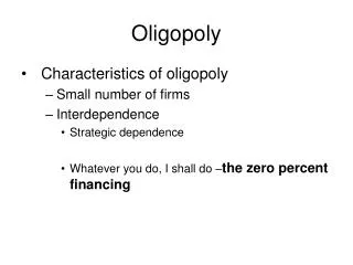
Characteristics of Oligopoly • Small number of firms • Product differentiation may or may not exist • Barriers to entry • Natural • Scale economies • Patents • Technology • Name recognition • Strategic action • Flooding the market • Controlling an essential input
Equilibrium in a Oligopolistic Market • In oligopoly the producers must consider the response of competitors when choosing output and price. • Defining Cournot-Nash Equilibrium • Equilibrium: Firms do the best they can and have no incentive to change their output or price • Cournot-Nash Equilibrium: Each firm is doing the best it can, given what its competitors are doing
A non-trivial example • Demand curve: P = 500 – 0.5X, where X = X1 + X2 • AC1 = MC1 =100; AC2 = MC2 = 150 • Can the second fellow survive if there is price competition? • Can he survive if there is quantity competition as in Cournot-Nash model? • TR1 = (500 – 0.5X).X1 = 500X1 – 0.5(X1 + X2)X1 = 500 -0.5X12 – 0.5X1.X2 => MR1 = dTR1/dX1 = 500 – 2.(1/2).X1 – 0.5X2 – 0.5X1.(dX2/dX1) = 500 – X1 -0.5X2, assuming conjectural variation =dX2/dX1 =0
Π-maximization by firms I & II • MR1 = MC1 => 500 – X1 – 0.5X2 = 100 => X1 = 400 -0.5X2 ----(a) giving the reaction function of firm 1, i.e., profit-maximizing value of X1 as function of X2. • (a) => If X1 = 0, then X2 = 800; If X2 =0, then X1 = 400 • Similarly, MR2 = MC2 gives 500 –X2 -0.5X1 = 150 => X2 = 350 -0.5X1 ---(b), giving the reaction function of firm 2 • (b) => If X1 =0, then X2 = 350; If X2 =0, then X1 = 700
Situation 1: Cournot-Nash Equilibrium • Both firms are dormant (followers): • (a) & (b) => X1=300; X2=200; X=500; P=250; Π1=45,000; Π2=20,000; Π=65,000; Thus firm-2 in profit, though relatively inefficient. X2 Collusive solution: Max Π=(500-0.5x)x – 100x =400x – 0.5x2 => dΠ/dx = 400 –x =0 =>x=400. Why is this solution lying on Firm 1’s reaction curve (a) where X1=400 and X2=0? 800 (a) Attempting a competitive solution with MC1=AC1=100 & MC2=AC2=150: Firm-2 thrown out in equilibrium and firm-1 will charge price P=150-ε, which is marginally less than 150 to prevent firm-2 from surfacing. Thus, P=500 – 0.5x1 =>150 = 500 – 0.5x1 => x1 =700. Why is it lying on firm-2’s reaction curve (b)? Is it more meaningful to call it a monopoly solution or a contestable market solution? 350 (c) 200 (b) 125 450 300 X1 400 533 700
Situation 2 (Stackelberg): Firm I active (leader), Firm II dormant (follower) • Now firm 1 sets dX2/dx1=-1/2, as picked up from firm II’s reaction function (b) • Then MR1=MC1 => 500 –X1 -0.5(X2 – 0.5X1) = 100 => 500 -3/4X1 -1/2X2 =100 => 400 = 3/4X1 + 1/2X2 => 3X1 +2X2 =400.4 => X1 = 400.4/3 – 2/3X2 ------(c), new reaction function of firm I • Solving (b) & (c) gives • X1=450; X2=125; X=575 • P=212.5 • Π1=50,625; Π2=7,812; Π=58,437 Thus, increase in intensity of competition increases output & reduces price; leader increases his market share.
Situation 3 (Stackelberg): Firm II active (leader), Firm I dormant (follower) • Now MR2 = 500 –X2 -0.5(X1 + (dX1/dX2).X2) = 500 -3/4X2 – ½ X1 • Hence MR2=MC2 => 500 -3/4X2 – ½ X1 = 150 => X2 = 1400/3 – 2/3X1 ------(d), new reaction function of firm II • Solving (a) & (d) gives • X1=250; X2=300; X=550 • P=225 • Π1=31,250; Π2=22,500; Π=53,750 Thus, the relatively inefficient firm II increases market share & profit (though still less than that of firm I in absolute terms). Lesson: Can we allow our generally inefficient PSUs to compete?
Situation 4 (Stackelberg): Both firms active (leaders) • Here we can check that • X1=400; X2=200; X=600 • P=200 • Π1=40,000; Π2=10,000; Π=50,000 • Thus, even larger total output at even lower price
All 4 situations put together in game theory format Player 1Player 2 Dormant Active Dormant 45,000; 20,000 31,250; 22,500 Active 50,625; 7,812 40,000; 10,000 To become active thus becomes the dominant strategy for both players
Text book example of Cournot Equilibrium • Market demand is P = 30 - Q where Q = Q1 + Q2 • Assumption of MC1 = MC2 = 0 has a limitation not merely because it is trivially fixed at zero, but also because MCs are equal • Firm 1’s Reaction Curve:
30 Firm 2’s Reaction Curve Cournot Equilibrium 15 10 Firm 1’s Reaction Curve 10 15 30 Textbook Duopoly Example Q1 The demand curve is P = 30 - Q and both firms have 0 marginal cost. a Is it a stable equilibrium? c d Q2 b Doesn’t stability of Cournot equilibrium betray its own assumption?
First Mover Advantage--The Stackelberg Model • Assumptions • One firm can set output first • MC = 0 as a simplifying assumption • Market demand is P = 30 - Q where Q = total output • Firm 1 sets output first and Firm 2 then makes an output decision
First Mover Advantage--The Stackelberg Model • Firm 1 • Must consider the reaction of Firm 2 • Firm 2 • Takes Firm 1’s output as fixed and therefore determines output with the Cournot reaction curve: Q2 = 15 - 1/2Q1
First Mover Advantage--The Stackelberg Model • Firm 1 • Choose Q1so that:
First Mover Advantage--The Stackelberg Model • Substituting Firm 2’s Reaction Curve for Q2: • Conclusion • Firm 1’s output is twice as large as firm 2’s • Firm 1’s profit is twice as large as firm 2’s
Why first-mover advantage? • First-mover’s output would be large. • If second-mover too produces a large output, then prices are driven down, causing loss to both. • If however, the second-mover produces a small output, then both firms make profits, but the first-mover makes larger profits corresponding to his larger output. • Since a rational second-mover values profits higher than revenge, he will set a small output, and both firms profit.
Firm 2’s Reaction Curve For the firm, collusion is the best outcome, followed by the Cournot equilibrium and then the competitive equilibrium Competitive Equilibrium (P = MC; Profit = 0) 15 Cournot Equilibrium Collusive Equilibrium 10 7.5 Firm 1’s Reaction Curve Collusion Curve 7.5 10 15 Implications of the Duopoly Example in the text Q1 Why this is not the competitive equilibrium? 30 Q2 30